Start here: your first disease progress workflow

Kaique S. Alves

2026-05-17

library(epifitter)
library(dplyr)
library(ggplot2)
library(cowplot)
theme_set(cowplot::theme_half_open(font_size = 12))

What epifitter does

epifitter helps analyze plant disease progress curves (DPCs): repeated measurements of disease intensity through time. These curves are common in plant pathology because they connect epidemic development, host-pathogen biology, management effects, and quantitative summaries such as apparent infection rate and area under the disease progress curve.

This article is the shortest path to a complete workflow. You will:

• simulate a synthetic epidemic;
• fit canonical disease progress models;
• inspect fitted parameters and model rankings;
• plot observed and fitted disease progress curves;
• see how the same workflow extends to multiple epidemics.

The examples use simulated data so that the workflow is reproducible, but the same functions can be applied to observed disease incidence or severity data on a proportional scale.

A first epidemic

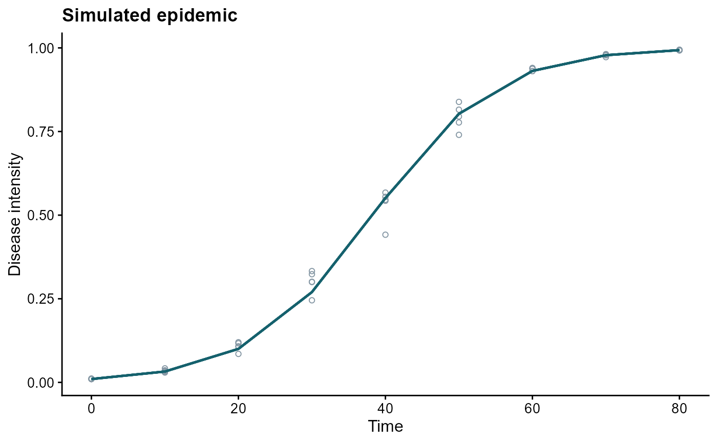
We start by simulating a logistic epidemic. The column y is the underlying curve and random_y represents replicated observations with sampling or measurement noise.

set.seed(1)

epi <- sim_logistic(
  N = 80,
  y0 = 0.01,
  dt = 10,
  r = 0.12,
  alpha = 0.2,
  n = 5
)

knitr::kable(head(epi), digits = 4)

replicates	time	y	random_y
1	0	0.0100	0.0100
1	10	0.0325	0.0336
1	20	0.1002	0.0851
1	30	0.2699	0.3328
1	40	0.5511	0.5674
1	50	0.8030	0.7770

ggplot(epi, aes(time, y, group = replicates)) +
  geom_point(aes(y = random_y), shape = 1, color = "#8597a4") +
  geom_line(color = "#15616d", linewidth = 0.8) +
  labs(
    title = "Simulated epidemic",
    x = "Time",
    y = "Disease intensity"
  )

Fit candidate models

fit_lin() compares the four canonical disease progress models by fitting linearized forms of each model. This is useful for quick screening and teaching, but the ranking should be interpreted together with the plot and biological plausibility.

fit <- fit_lin(time = epi$time, y = epi$random_y)
fit

## Results of fitting population models 
## 
## Stats:
##                  CCC r_squared    RSE
## Logistic      0.9988    0.9976 0.1561
## Gompertz      0.9774    0.9558 0.4734
## Monomolecular 0.9313    0.8714 0.6420
## Exponential   0.9161    0.8452 0.6337
## 
##  Infection rate:
##                 Estimate    Std.error      Lower      Upper
## Logistic      0.11931599 0.0009014682 0.11749801 0.12113397
## Gompertz      0.08329917 0.0027332800 0.07778699 0.08881135
## Monomolecular 0.06325781 0.0037064427 0.05578306 0.07073257
## Exponential   0.05605817 0.0036589168 0.04867927 0.06343708
## 
##  Initial inoculum:
##                    Estimate Linearized     lin.SE         Lower        Upper
## Logistic       1.058484e-02 -4.5376913 0.04291847  9.715742e-03  0.011530776
## Gompertz       7.809693e-05 -2.2468144 0.13013015  4.571513e-06  0.000692952
## Monomolecular -1.515280e+00 -0.9223841 0.17646197 -2.590364e+00 -0.762114625
## Exponential    2.690866e-02 -3.6153072 0.17419928  1.893746e-02  0.038235118

fit$stats_all contains the full ranking of candidate models.

knitr::kable(fit$stats_all, digits = 4)

best_model	model	r	r_se	r_ci_lwr	r_ci_upr	v0	v0_se	r_squared	RSE	CCC	y0	y0_ci_lwr	y0_ci_upr
1	Logistic	0.1193	0.0009	0.1175	0.1211	-4.5377	0.0429	0.9976	0.1561	0.9988	0.0106	0.0097	0.0115
2	Gompertz	0.0833	0.0027	0.0778	0.0888	-2.2468	0.1301	0.9558	0.4734	0.9774	0.0001	0.0000	0.0007
3	Monomolecular	0.0633	0.0037	0.0558	0.0707	-0.9224	0.1765	0.8714	0.6420	0.9313	-1.5153	-2.5904	-0.7621
4	Exponential	0.0561	0.0037	0.0487	0.0634	-3.6153	0.1742	0.8452	0.6337	0.9161	0.0269	0.0189	0.0382

Visualize predictions

The fitted object stores observed values, transformed values, predictions, and parameter summaries. plot_fit() turns that object into a faceted ggplot2 figure.

plot_fit(fit, point_size = 1.8, line_size = 0.9)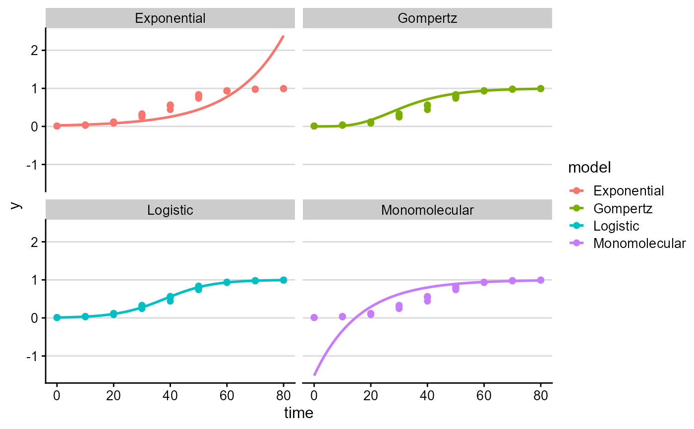

Work with multiple epidemics

Many experiments include multiple treatments, cultivars, blocks, or locations. Use fit_multi() when the same fitting workflow should be applied separately to each group.

epi_a <- sim_gompertz(N = 50, y0 = 0.002, dt = 5, r = 0.10, alpha = 0.2, n = 3)
epi_b <- sim_gompertz(N = 50, y0 = 0.002, dt = 5, r = 0.14, alpha = 0.2, n = 3)

multi_epi <- bind_rows(epi_a, epi_b, .id = "epidemic")

multi_fit <- fit_multi(
  time_col = "time",
  intensity_col = "random_y",
  data = multi_epi,
  strata_cols = "epidemic"
)

knitr::kable(head(multi_fit$Parameters), digits = 4)

epidemic	best_model	model	r	r_se	r_ci_lwr	r_ci_upr	v0	v0_se	r_squared	RSE	CCC	y0	y0_ci_lwr	y0_ci_upr
1	1	Gompertz	0.0997	0.0017	0.0962	0.1032	-1.7976	0.0513	0.9907	0.1575	0.9953	0.0024	0.0012	0.0044
1	2	Monomolecular	0.0671	0.0032	0.0605	0.0737	-0.4718	0.0957	0.9327	0.2939	0.9652	-0.6028	-0.9484	-0.3186
1	3	Logistic	0.1655	0.0090	0.1473	0.1838	-4.3343	0.2650	0.9168	0.8136	0.9566	0.0129	0.0076	0.0220
1	4	Exponential	0.0984	0.0115	0.0751	0.1218	-3.8625	0.3390	0.7042	1.0408	0.8264	0.0210	0.0105	0.0420
2	1	Gompertz	0.1404	0.0018	0.1367	0.1441	-1.7956	0.0537	0.9949	0.1648	0.9974	0.0024	0.0012	0.0045
2	2	Monomolecular	0.1102	0.0036	0.1028	0.1175	-0.6420	0.1069	0.9677	0.3282	0.9836	-0.9003	-1.3632	-0.5281

Next steps

• Use the PowderyMildew article for a real-data workflow based on the bundled experimental dataset.
• Use the model fitting article for a deeper walkthrough of fit_lin(), fit_nlin(), fit_nlin2(), weighted nonlinear fits, and fit_multi().
• Use the confidence interval article when you need uncertainty bands around fitted curves.
• Use the area-under-the-curve article when your goal is to summarize each epidemic as AUDPC or AUDPS.
• Use the simulation workflow article for examples built around the sim_ family.