Model fitting workflows

Kaique S. Alves

2026-04-11

library(epifitter)
library(dplyr)
library(ggplot2)
library(cowplot)
theme_set(cowplot::theme_half_open(font_size = 12))

Overview

epifitter offers three complementary fitting workflows:

• fit_lin() for linearized model comparison;
• fit_nlin() for nonlinear fitting of two-parameter models;
• fit_nlin2() for nonlinear fitting when the asymptote K should be estimated.

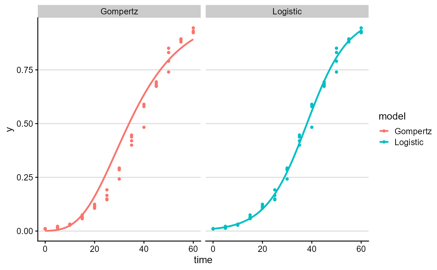
Compare models quickly with fit_lin()

set.seed(1)
epi <- sim_logistic(N = 60, y0 = 0.01, dt = 5, r = 0.12, alpha = 0.2, n = 4)

fit_lin_out <- fit_lin(time = epi$time, y = epi$random_y)
knitr::kable(fit_lin_out$stats_all, digits = 4)

best_model	model	r	r_se	r_ci_lwr	r_ci_upr	v0	v0_se	r_squared	RSE	CCC	y0	y0_ci_lwr	y0_ci_upr
1	Logistic	0.1202	0.0011	0.1180	0.1224	-4.5730	0.0394	0.9957	0.1504	0.9979	0.0102	0.0095	0.0111
2	Gompertz	0.0694	0.0022	0.0649	0.0739	-1.9893	0.0792	0.9505	0.3021	0.9746	0.0007	0.0002	0.0020
3	Exponential	0.0780	0.0029	0.0722	0.0839	-4.0617	0.1032	0.9346	0.3938	0.9662	0.0172	0.0140	0.0212
4	Monomolecular	0.0422	0.0028	0.0366	0.0478	-0.5113	0.0983	0.8215	0.3751	0.9020	-0.6674	-1.0315	-0.3687

plot_fit(fit_lin_out, models = c("Logistic", "Gompertz"))

Nonlinear fitting with starting values

fit_nlin_out <- fit_nlin(
  time = epi$time,
  y = epi$random_y,
  starting_par = list(y0 = 0.01, r = 0.03)
)

fit_nlin_out$stats_all

Estimate K when the epidemic plateaus below 1

epi_partial <- epi %>%
  mutate(random_y = random_y * 0.8)

fit_k <- fit_nlin2(
  time = epi_partial$time,
  y = epi_partial$random_y,
  starting_par = list(y0 = 0.01, r = 0.03, K = 0.7)
)

fit_k$stats_all

Grouped fitting with fit_multi()

epi1 <- sim_gompertz(N = 50, y0 = 0.001, dt = 5, r = 0.08, alpha = 0.2, n = 3)
epi2 <- sim_gompertz(N = 50, y0 = 0.002, dt = 5, r = 0.11, alpha = 0.2, n = 3)

multi_epi <- bind_rows(epi1, epi2, .id = "curve")

multi_fit <- fit_multi(
  time_col = "time",
  intensity_col = "random_y",
  data = multi_epi,
  strata_cols = "curve"
)

knitr::kable(head(multi_fit$Parameters), digits = 4)

curve	best_model	model	r	r_se	r_ci_lwr	r_ci_upr	v0	v0_se	r_squared	RSE	CCC	y0	y0_ci_lwr	y0_ci_upr
1	1	Gompertz	0.0813	0.0016	0.0780	0.0846	-1.9382	0.0480	0.9878	0.1475	0.9939	0.0010	0.0005	0.0018
1	2	Logistic	0.1623	0.0091	0.1438	0.1808	-5.1753	0.2685	0.9116	0.8244	0.9537	0.0056	0.0033	0.0097
1	3	Monomolecular	0.0449	0.0026	0.0396	0.0502	-0.3618	0.0769	0.9058	0.2360	0.9506	-0.4359	-0.6796	-0.2276
1	4	Exponential	0.1174	0.0111	0.0948	0.1400	-4.8135	0.3276	0.7838	1.0058	0.8788	0.0081	0.0042	0.0158
2	1	Gompertz	0.1126	0.0015	0.1095	0.1157	-1.8561	0.0448	0.9944	0.1377	0.9972	0.0017	0.0009	0.0029
2	2	Monomolecular	0.0802	0.0035	0.0729	0.0874	-0.5657	0.1050	0.9427	0.3224	0.9705	-0.7606	-1.1810	-0.4212

knitr::kable(head(multi_fit$Data), digits = 4)

curve	time	y	model	linearized	predicted	residual
1	0	0.0011	Exponential	-6.8418	0.0081	-0.0071
1	0	0.0011	Monomolecular	0.0011	-0.4359	0.4370
1	0	0.0011	Logistic	-6.8408	0.0056	-0.0046
1	0	0.0011	Gompertz	-1.9231	0.0010	0.0001
1	5	0.0076	Exponential	-4.8831	0.0146	-0.0070
1	5	0.0076	Monomolecular	0.0076	-0.1473	0.1549