Plot fitted epidemic models — plot

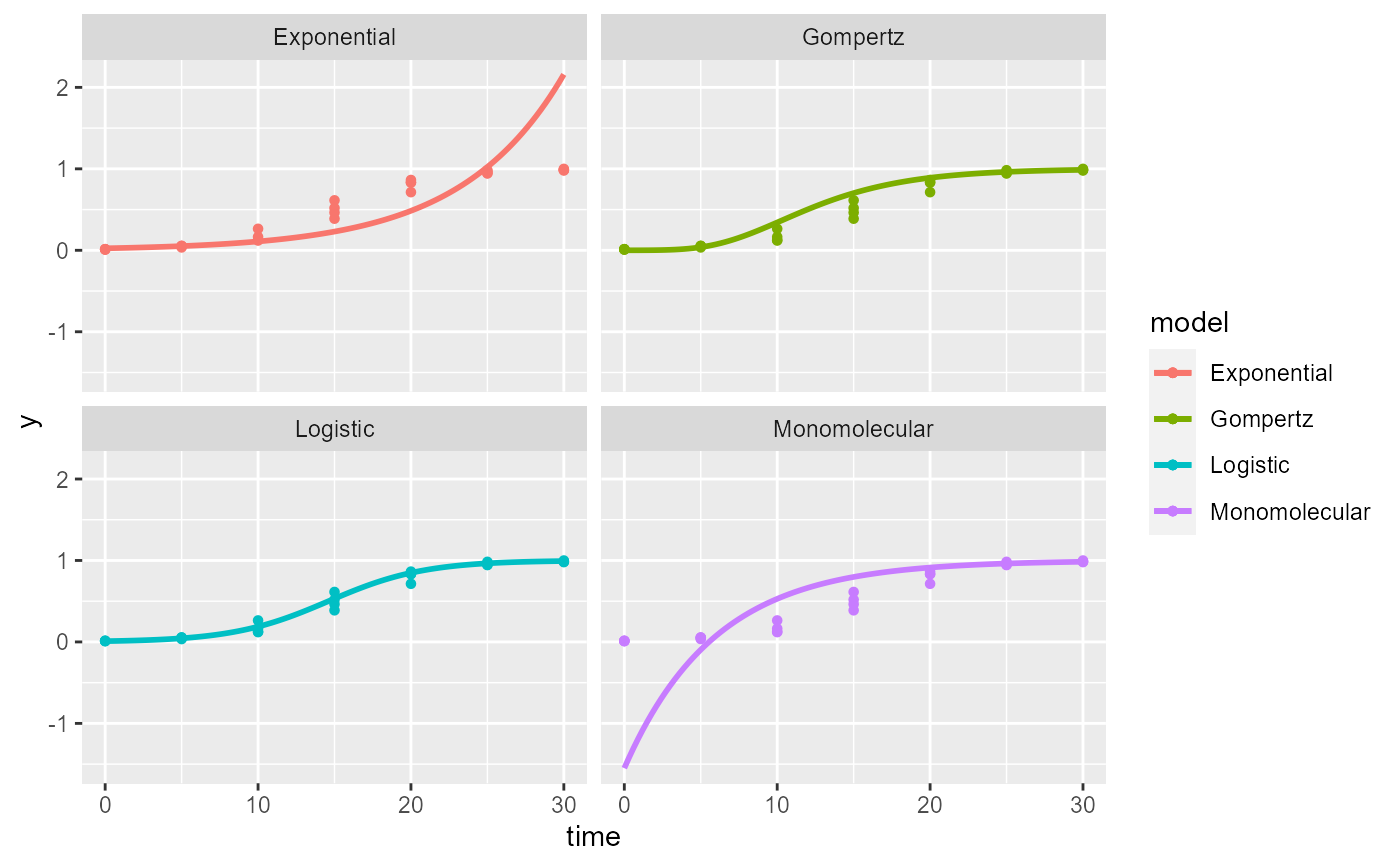
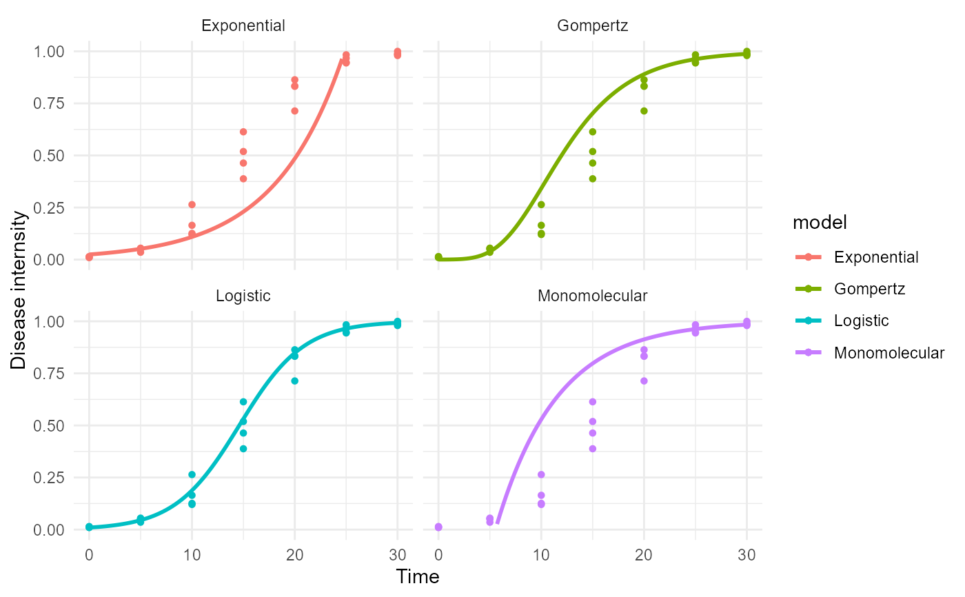
Create a faceted `ggplot2` panel showing observed and fitted values for the selected epidemic models. Optionally, add confidence bands around the fitted curves.

Usage

plot_fit(
  object,
  point_size = 1.2,
  line_size = 1,
  models = c("Exponential", "Monomolecular", "Logistic", "Gompertz"),
  conf_int = FALSE,
  ci_method = c("bootstrap", "wild"),
  nsim = 500,
  level = 0.95,
  seed = NULL,
  n_grid = 100,
  ci_alpha = 0.2,
  y_bounds = c(0, 1)
)

Arguments

object: A fitted object returned by `fit_lin()`, `fit_nlin()`, or `fit_nlin2()`.
point_size: Point size for observed values.
line_size: Line width for fitted curves.
models: Character vector with the models to display.
conf_int: Logical. If `TRUE`, draw confidence bands around fitted curves.
ci_method: Method used to estimate confidence bands. Use `"bootstrap"` for residual bootstrap intervals, or `"wild"` for wild residual bootstrap intervals. The older `"case"` option is accepted as a deprecated alias for `"wild"`.
nsim: Number of bootstrap samples used when `conf_int = TRUE`.
level: Confidence level for the interval.
seed: Optional random seed used for interval estimation.
n_grid: Number of time points used to draw fitted curves and confidence bands.
ci_alpha: Transparency of the confidence band.
y_bounds: Numeric vector of length two used to constrain plotted fitted values and confidence bands. The default keeps disease intensity on the usual proportion scale from 0 to 1. Use `NULL` to show unconstrained fitted values.

Value

A `ggplot2` object.

Examples

epi <- sim_logistic(N = 30, y0 = 0.01, dt = 5, r = 0.3, alpha = 0.2, n = 4)
fit <- fit_lin(time = epi$time, y = epi$random_y)
plot_fit(fit)

# \donttest{
plot_fit(fit, conf_int = TRUE, nsim = 100)

# }