Simulation workflows

Kaique S. Alves

2026-04-11

library(epifitter)
library(ggplot2)
library(cowplot)
theme_set(cowplot::theme_half_open(font_size = 12))

Overview

The sim_ family creates synthetic disease progress curves that match the same model families used by the fitting functions.

Simulate four canonical curve shapes

exp_model <- sim_exponential(N = 100, y0 = 0.01, dt = 10, r = 0.045, alpha = 0.2, n = 5)
mono_model <- sim_monomolecular(N = 100, y0 = 0.01, dt = 5, r = 0.05, alpha = 0.2, n = 5)
log_model <- sim_logistic(N = 100, y0 = 0.01, dt = 5, r = 0.10, alpha = 0.2, n = 5)
gomp_model <- sim_gompertz(N = 100, y0 = 0.01, dt = 5, r = 0.07, alpha = 0.2, n = 5)

exp_plot <- ggplot(exp_model, aes(time, y)) +
  geom_jitter(aes(y = random_y), width = 0.1, color = "#6c757d") +
  geom_line(color = "#b56576", linewidth = 0.8) +
  labs(title = "Exponential")

mono_plot <- ggplot(mono_model, aes(time, y)) +
  geom_jitter(aes(y = random_y), width = 0.1, color = "#6c757d") +
  geom_line(color = "#588157", linewidth = 0.8) +
  labs(title = "Monomolecular")

log_plot <- ggplot(log_model, aes(time, y)) +
  geom_jitter(aes(y = random_y), width = 0.1, color = "#6c757d") +
  geom_line(color = "#355070", linewidth = 0.8) +
  labs(title = "Logistic")

gomp_plot <- ggplot(gomp_model, aes(time, y)) +
  geom_jitter(aes(y = random_y), width = 0.1, color = "#6c757d") +
  geom_line(color = "#8d5a97", linewidth = 0.8) +
  labs(title = "Gompertz")

plot_grid(exp_plot, mono_plot, log_plot, gomp_plot, ncol = 2)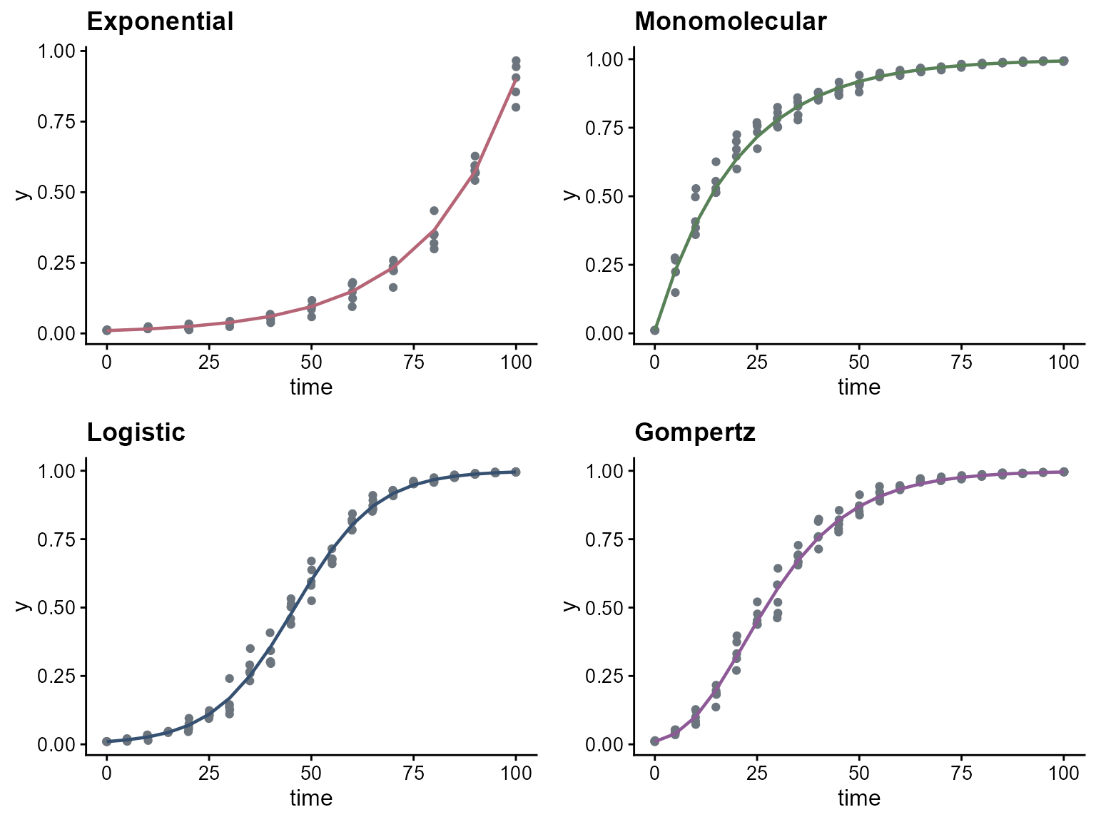

Send simulated data into the fitting pipeline

fit_from_sim <- fit_lin(time = log_model$time, y = log_model$random_y)
fit_from_sim$stats_all

## # A tibble: 4 × 14
##   best_model model      r    r_se r_ci_lwr r_ci_upr    v0  v0_se r_squared   RSE
##        <int> <chr>  <dbl>   <dbl>    <dbl>    <dbl> <dbl>  <dbl>     <dbl> <dbl>
## 1          1 Logi… 0.101  6.96e-4   0.0998   0.103  -4.65 0.0407     0.995 0.216
## 2          2 Gomp… 0.0723 1.50e-3   0.0694   0.0753 -2.41 0.0879     0.957 0.467
## 3          3 Mono… 0.0559 2.02e-3   0.0519   0.0599 -1.10 0.118      0.881 0.628
## 4          4 Expo… 0.0453 1.99e-3   0.0413   0.0492 -3.55 0.116      0.834 0.617
## # ℹ 4 more variables: CCC <dbl>, y0 <dbl>, y0_ci_lwr <dbl>, y0_ci_upr <dbl>