Area-under-the-curve summaries

library(epifitter)
library(ggplot2)
library(dplyr)
library(cowplot)
theme_set(cowplot::theme_half_open(font_size = 12))

Overview

Area-under-the-curve summaries are useful when the goal is to condense an entire disease progress curve into a single number that represents epidemic intensity over time.

epifitter currently provides three related functions:

AUDPC() for the area under the disease progress curve.
AUDPC_2_points() for estimating AUDPC from just two observations under a logistic assumption.
AUDPS() for the area under the disease progress stairs, which gives more balanced weight to the first and last observations.

For AUDPC() and AUDPS(), repeated observations at the same time point are now handled explicitly through the aggregate argument. By default, replicated observations are averaged per time point before the area is calculated.

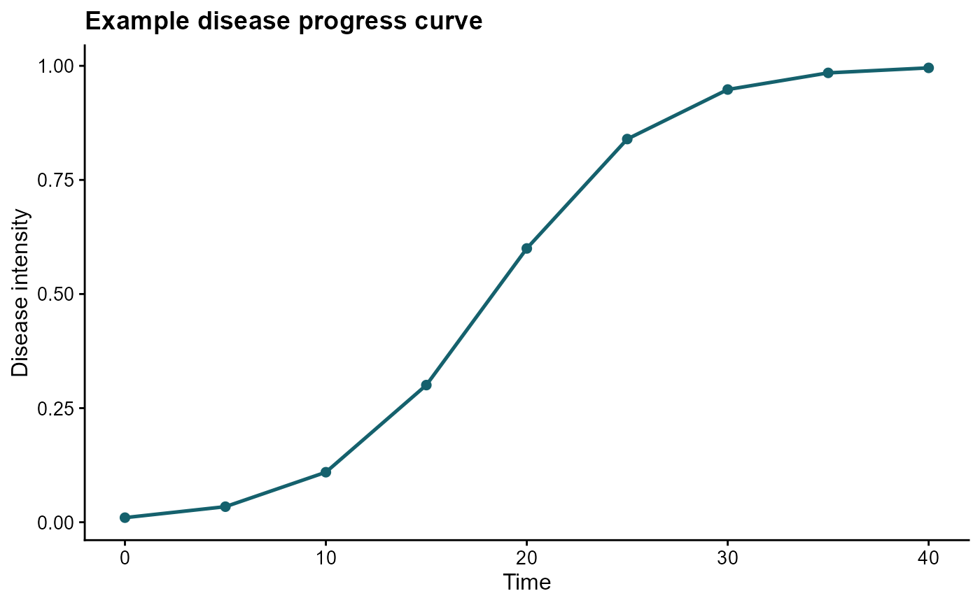
Build an example curve

We start with a simulated epidemic and use the disease intensity values across time.

set.seed(1)

epi <- sim_logistic(
  N = 40,
  y0 = 0.01,
  dt = 5,
  r = 0.25,
  alpha = 0.2,
  n = 1
)

knitr::kable(epi, digits = 4)

replicates	time	y	random_y
1	0	0.0100	0.0100
1	5	0.0341	0.0353
1	10	0.1096	0.0933
1	15	0.3005	0.3675
1	20	0.5999	0.6157
1	25	0.8396	0.8175
1	30	0.9481	0.9529
1	35	0.9846	0.9868
1	40	0.9955	0.9960

ggplot(epi, aes(time, y)) +
  geom_point(size = 2, color = "#15616d") +
  geom_line(linewidth = 0.9, color = "#15616d") +
  labs(
    title = "Example disease progress curve",
    x = "Time",
    y = "Disease intensity"
  )

Line plot of a simulated disease progress curve showing disease intensity increasing over time.

Compute AUDPC

AUDPC() uses the trapezoidal method to summarize the curve over the observed period.

audpc_abs <- AUDPC(
  time = epi$time,
  y = epi$y,
  y_proportion = TRUE,
  type = "absolute"
)

audpc_abs

## [1] 21.62241

When the interest is in a scale-free measure, use type = "relative".

audpc_rel <- AUDPC(
  time = epi$time,
  y = epi$y,
  y_proportion = TRUE,
  type = "relative"
)

audpc_rel

## [1] 0.5405602

The relative version is useful for comparing epidemics observed over the same time span but with different scales.

Multiple observations at the same time

Many experiments include replicated plots assessed on the same dates. In that setting, the area summary should be computed from one value per time point, not from the raw row order.

By default, AUDPC() and AUDPS() aggregate replicated observations using the mean at each time.

time_rep <- c(0, 0, 5, 5, 10, 10)
y_rep <- c(0.10, 0.30, 0.40, 0.60, 0.70, 0.90)

AUDPC(time = time_rep, y = y_rep)

## [1] 5.75

AUDPS(time = time_rep, y = y_rep)

## [1] 8.25

This is equivalent to calculating the area from the per-time means.

time_mean <- c(0, 5, 10)
y_mean <- c(mean(c(0.10, 0.30)), mean(c(0.40, 0.60)), mean(c(0.70, 0.90)))

AUDPC(time = time_mean, y = y_mean, aggregate = "none")

## [1] 5.75

AUDPS(time = time_mean, y = y_mean, aggregate = "none")

## [1] 8.25

If a more robust summary is preferred, use the median instead of the mean.

AUDPC(time = time_rep, y = y_rep, aggregate = "median")

## [1] 5.75

AUDPS(time = time_rep, y = y_rep, aggregate = "median")

## [1] 8.25

If you want to require unique time values and catch duplicated assessments as an error, set aggregate = "none".

AUDPC(time = time_rep, y = y_rep, aggregate = "none")
AUDPS(time = time_rep, y = y_rep, aggregate = "none")

One summary curve versus one value per replicate

This distinction is important in experimental data.

If you pass all replicated observations together to AUDPC() or AUDPS(), the functions now assume you want a single summary curve, and they aggregate the repeated observations at each time point before computing the area.

If instead you want one AUDPC or AUDPS value for each experimental replicate, compute the area separately within each replicate.

epi_rep <- sim_logistic(
  N = 30,
  y0 = 0.01,
  dt = 5,
  r = 0.3,
  alpha = 0.2,
  n = 4
)

knitr::kable(head(epi_rep), digits = 4)

replicates	time	y	random_y
1	0	0.0100	0.0100
1	5	0.0433	0.0558
1	10	0.1687	0.1796
1	15	0.4763	0.4453
1	20	0.8030	0.7329
1	25	0.9481	0.9592

A single treatment-level summary can be obtained by pooling all rows and using the default aggregation by time:

AUDPC(time = epi_rep$time, y = epi_rep$random_y)

## [1] 14.70536

AUDPS(time = epi_rep$time, y = epi_rep$random_y)

## [1] 17.20195

To obtain one value per replicate, group the data and compute the areas within each experimental unit. In this case, use aggregate = "none" because each replicate should contribute only one observation per time point.

epi_rep %>%
  group_by(replicates) %>%
  summarise(
    audpc = AUDPC(time = time, y = random_y, aggregate = "none"),
    audps = AUDPS(time = time, y = random_y, aggregate = "none"),
    .groups = "drop"
  ) %>%
  knitr::kable(digits = 4)

replicates	audpc	audps
1	14.4302	16.9247
2	15.2590	17.7543
3	14.5306	17.0279
4	14.6017	17.1009

In practice:

use the default aggregation when you want one area summary for the mean epidemic across replicates;
group by replicate when you want one area summary per experimental unit.

Compute AUDPS

AUDPS() is closely related to AUDPC(), but uses a staircase correction that often improves discrimination among curves in comparative studies.

audps_abs <- AUDPS(
  time = epi$time,
  y = epi$y,
  y_proportion = TRUE,
  type = "absolute"
)

audps_abs

## [1] 24.13622

audps_rel <- AUDPS(
  time = epi$time,
  y = epi$y,
  y_proportion = TRUE,
  type = "relative"
)

audps_rel

## [1] 0.5363605

Estimate AUDPC from two observations

AUDPC_2_points() is helpful when only the initial and final disease intensities are available and a logistic epidemic shape is assumed.

audpc_two_points <- AUDPC_2_points(
  time = epi$time[7],
  y0 = epi$y[1],
  yT = epi$y[7]
)

audpc_two_points

## [1] 11.79275

For simulated logistic data, this estimate should be close to the full-curve AUDPC computed from all intermediate observations.

full_curve_audpc <- AUDPC(
  time = epi$time,
  y = epi$y,
  y_proportion = TRUE
)

c(
  AUDPC_full_curve = full_curve_audpc,
  AUDPC_two_points = audpc_two_points
)

## AUDPC_full_curve AUDPC_two_points 
##         21.62241         11.79275

Absolute versus relative measures

Use absolute values when duration and measurement scale are already part of the interpretation.

Use relative values when you want a normalized measure between epidemics observed on the same conceptual scale.

Practical guidance

Use AUDPC() as the standard summary for cumulative disease burden.
Use AUDPS() when endpoint weighting matters and you want an alternative to the trapezoidal summary.
Use AUDPC_2_points() only when two observations are available and the logistic assumption is justified.
When you have replicated observations at the same time point, keep the default aggregate = "mean" or choose aggregate = "median" explicitly.
When you need one value per replicate or plot, calculate the summaries inside each group and use aggregate = "none" within that group.

Kaique S. Alves

2026-04-11