Uncertainty bands for fitted disease progress curves

library(epifitter)

Why add intervals?

Fitted disease progress curves are usually shown as a single line, but the line is only an estimate. Confidence bands help communicate the uncertainty around the fitted epidemic curve.

This article focuses on uncertainty in the fitted mean curve. The bands shown by plot_fit() are not prediction intervals for future observations, and they do not replace a full model-based analysis of treatment effects. They are a visual tool for asking how stable the fitted curve is under residual resampling.

In epifitter, confidence bands are added directly in plot_fit():

plot_fit(fit, conf_int = TRUE, ci_method = "bootstrap", nsim = 500)

The argument conf_int controls whether the interval is drawn. The argument ci_method controls how the interval is estimated.

Use these intervals to compare fitted shapes cautiously. If the scientific question is a formal comparison among treatments, use a statistical model that matches the experimental design after defining the target quantity.

Example data

We first simulate one logistic epidemic with moderate observational noise and fit the four linearized epidemic models. The noise is intentionally visible in this example so the confidence bands are easy to inspect.

set.seed(123)

epi <- sim_logistic(
  N = 30,
  y0 = 0.01,
  dt = 5,
  r = 0.25,
  alpha = 0.40,
  n = 1
)

fit <- fit_lin(time = epi$time, y = epi$random_y)

head(fit$data)
#>   time          y         model  linearized     predicted      residual
#> 1    0 0.01000000   Exponential -4.60517019  0.0184182273 -8.418227e-03
#> 2    0 0.01000000 Monomolecular  0.01005034 -0.8327456690  8.427457e-01
#> 3    0 0.01000000      Logistic -4.59511985  0.0099495389  5.046107e-05
#> 4    0 0.01000000      Gompertz -1.52717963  0.0004464615  9.553538e-03
#> 5    5 0.03102984   Exponential -3.47280593  0.0400754198 -9.045579e-03
#> 6    5 0.03102984 Monomolecular  0.03152146 -0.0538461759  8.487602e-02

Residual bootstrap confidence bands

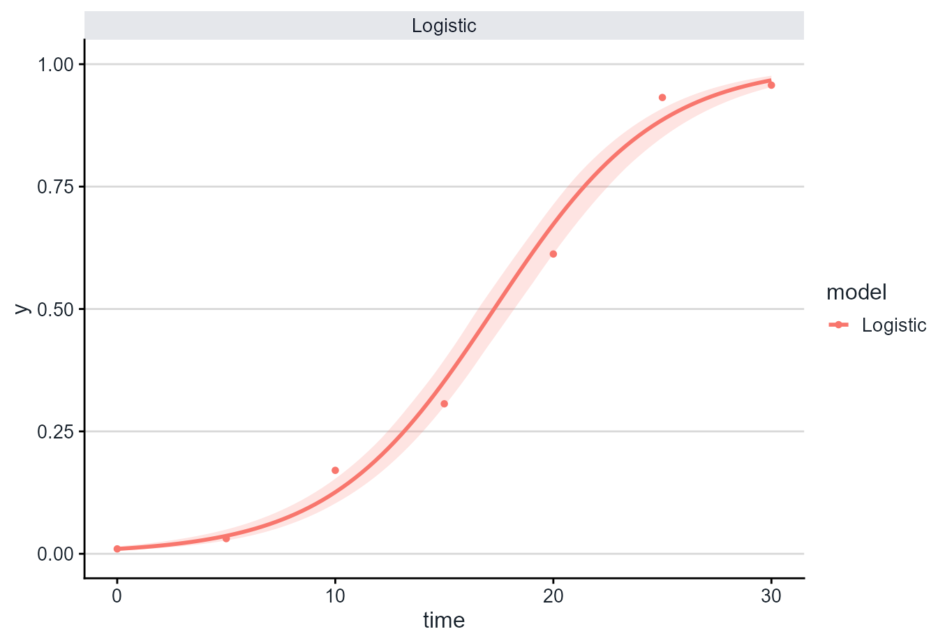
The default bootstrap method resamples residuals from the fitted curve, creates new plausible disease progress curves at the observed assessment times, refits the model many times, and builds the band from the distribution of fitted curves.

This approach assumes that the residual pattern is a reasonable basis for generating plausible alternative curves. It is useful for visualization, but it should still be checked against the biology of the system and the assessment design.

plot_fit(
  fit,
  models = "Logistic",
  conf_int = TRUE,
  ci_method = "bootstrap",
  nsim = 100,
  seed = 123
)

For final analyses, increase nsim, for example:

plot_fit(fit, conf_int = TRUE, ci_method = "bootstrap", nsim = 500)

Larger values of nsim make the interval more stable, but also make the plot slower to compute.

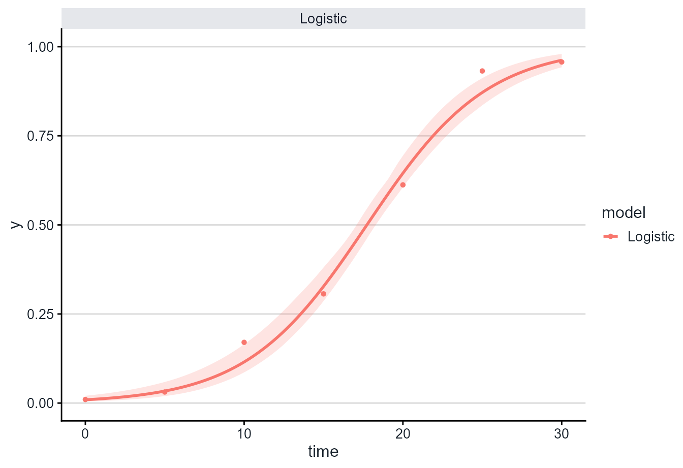
Wild bootstrap confidence bands

The wild bootstrap method randomly changes the sign of resampled residuals before refitting the model. This keeps the original assessment times intact and is available with ci_method = "wild".

Wild bootstrap intervals are often useful as a sensitivity check when residual variation changes across the range of fitted values.

plot_fit(
  fit,
  models = "Logistic",
  conf_int = TRUE,
  ci_method = "wild",
  nsim = 100,
  seed = 123
)

Compare multiple models

Confidence bands can also be drawn for more than one model at a time.

plot_fit(
  fit,
  models = c("Exponential", "Logistic", "Gompertz"),
  conf_int = TRUE,
  ci_method = "bootstrap",
  nsim = 100,
  seed = 123,
  y_bounds = NULL
)

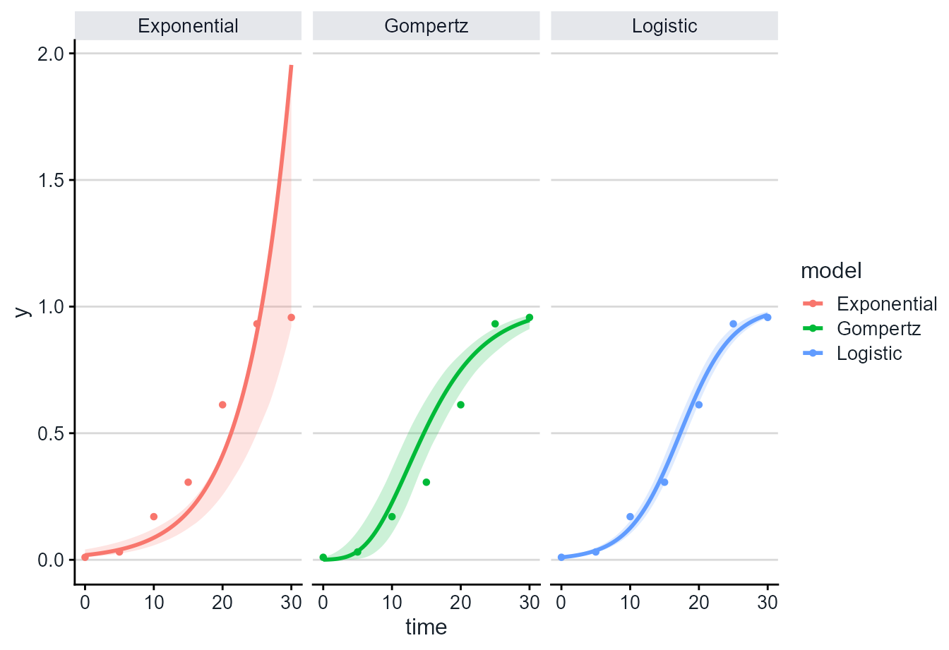
Here y_bounds = NULL leaves fitted values on their natural model scale. This is useful when comparing model forms because the exponential model can extrapolate above 1, which is a warning sign when disease intensity is a proportion. The fitted curve also does not have to sit in the middle of the band: bootstrap intervals are built from quantiles of refitted curves, so they can be asymmetric when the model is nonlinear or poorly matched to the data.

Nonlinear fits

The same interface works with nonlinear fits returned by fit_nlin() and fit_nlin2().

nlin_fit <- fit_nlin(
  time = epi$time,
  y = epi$random_y,
  starting_par = list(y0 = 0.01, r = 0.1),
  maxiter = 200
)
#> Warning: The following nonlinear model(s) did not converge and will be returned
#> as NA: Monomolecular.

plot_fit(
  nlin_fit,
  models = "Logistic",
  conf_int = TRUE,
  ci_method = "bootstrap",
  nsim = 100,
  seed = 123
)

Choosing a method

Use ci_method = "bootstrap" for the main fitted-curve intervals. Use ci_method = "wild" as a sensitivity check when you want a second residual bootstrap strategy that preserves the original assessment times.

In very smooth datasets, the confidence band may be narrow. Wider bands usually appear when the observations are noisier, when there are fewer assessment times, or when the fitted model is less certain.

In both cases, level controls the confidence level:

plot_fit(fit, conf_int = TRUE, ci_method = "bootstrap", level = 0.90)
plot_fit(fit, conf_int = TRUE, ci_method = "bootstrap", level = 0.95)

The bands shown by plot_fit() are confidence bands for the fitted curve, not prediction intervals for future observations.

Report nsim, level, the fitting method, and the interval method when using these plots in reports or manuscripts.

By default, plot_fit() keeps fitted curves and bands on the disease proportion scale from 0 to 1. To inspect unconstrained fitted values, use:

plot_fit(fit, conf_int = TRUE, y_bounds = NULL)