Compare EC50 models
Kaique S Alves
2026-05-24
Source:vignettes/ec50_multimodel.Rmd
ec50_multimodel.RmdWhen to Use This Workflow
Use ec50_multimodel() when you need to compare candidate
dose-response models before reporting EC50 estimates. The function fits
each model within each isolate and stratum, stores the fitted
drc objects, and returns a data frame with EC50 estimates
plus model-selection statistics.
Packages and Data
data(multi_isolate)

example_data <- subset(
  multi_isolate,
  isolate %in% 1:5 & fungicida == "Fungicide A"
)

head(example_data)
## isolate field fungicida dose growth
## 1 1 Organic Fungicide A 0e+00 20.2082399
## 2 1 Organic Fungicide A 1e-05 20.1168279
## 3 1 Organic Fungicide A 1e-04 19.2479678
## 4 1 Organic Fungicide A 1e-03 15.8123455
## 5 1 Organic Fungicide A 1e-02 7.3206757
## 6 1 Organic Fungicide A 1e-01 0.6985264Inspect the Raw Pattern
Repeated observations at the same dose should be shown as points, not connected with lines. Lines are reserved for fitted model curves. The exploratory plot below uses positive doses because the x-axis is log-scaled.
raw_plot_data <- subset(example_data, dose > 0)

ggplot(raw_plot_data, aes(dose, growth, color = factor(isolate))) +
  geom_jitter(width = 0.08, height = 0, alpha = 0.85, size = 2) +
  facet_wrap(~field) +
  scale_x_log10() +
  labs(x = "Dose", y = "Growth", color = "Isolate") +
  theme_light()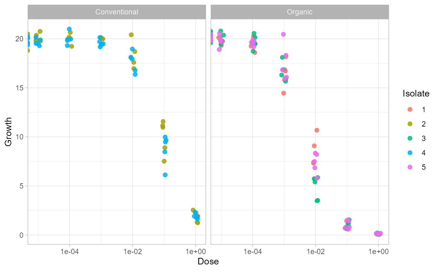
Check the Data
Use check_ec50_data() before model fitting. The returned
flags help separate data problems from model-fitting problems.
check_ec50_data(
  example_data,
  response = "growth",
  dose = "dose",
  isolate = "isolate",
  strata = "field"
)
## ID field n_obs n_doses missing_response missing_dose nonpositive_dose
## 1 1 Organic 35 7 0 0 5
## 2 2 Conventional 35 7 0 0 5
## 3 3 Organic 35 7 0 0 5
## 4 4 Conventional 35 7 0 0 5
## 5 5 Organic 35 7 0 0 5
## duplicated_rows no_response_variation too_few_observations too_few_doses
## 1 0 FALSE FALSE FALSE
## 2 0 FALSE FALSE FALSE
## 3 0 FALSE FALSE FALSE
## 4 0 FALSE FALSE FALSE
## 5 0 FALSE FALSE FALSEFit Candidate Models
Pass a named or unnamed list of drc model functions to
fct. The fitted object keeps the EC50 estimates as rows and
stores the fitted models for downstream helpers.
fit <- ec50_multimodel(
  growth ~ dose,
  data = example_data,
  isolate_col = "isolate",
  strata_col = "field",
  fct = list(drc::LL.3(), drc::LL.4(), drc::W2.3()),
  interval = "delta"
)

head(ec50_estimates(fit))
## ID field Estimate Std..Error Lower Upper logLik
## 1 1 Organic 0.006072082 0.0005740341 0.004902813 0.007241351 -45.15079
## 2 2 Conventional 0.101455765 0.0076364691 0.085900787 0.117010744 -43.53183
## 3 3 Organic 0.003776957 0.0002432571 0.003281459 0.004272456 -36.09845
## 4 4 Conventional 0.079971237 0.0055655891 0.068634503 0.091307971 -38.42154
## 5 5 Organic 0.006122508 0.0004575060 0.005190599 0.007054418 -41.41058
## 6 1 Organic 0.006364103 0.0007031475 0.004930024 0.007798182 -44.69257
## IC Lack.of.fit Res.var model
## 1 98.30158 0.7271292 0.8451681 LL.3
## 2 95.06365 0.9866424 0.7704874 LL.3
## 3 80.19689 0.3897432 0.5038400 LL.3
## 4 84.84309 0.8328859 0.5753664 LL.3
## 5 90.82115 0.9744433 0.6825317 LL.3
## 6 99.38515 0.7370811 0.8498845 LL.4Diagnose Fits
fit_quality() summarizes successful model fits.
fit_failures() returns failed group/model combinations as
data.
fit_quality(fit)## ID field model fit_status n_obs n_doses dose_min dose_max
## 1 1 Organic LL.3 ok 35 7 0 1
## 2 2 Conventional LL.3 ok 35 7 0 1
## 3 3 Organic LL.3 ok 35 7 0 1
## 4 4 Conventional LL.3 ok 35 7 0 1
## 5 5 Organic LL.3 ok 35 7 0 1
## 6 1 Organic LL.4 ok 35 7 0 1
## 7 2 Conventional LL.4 ok 35 7 0 1
## 8 3 Organic LL.4 ok 35 7 0 1
## 9 4 Conventional LL.4 ok 35 7 0 1
## 10 5 Organic LL.4 ok 35 7 0 1
## 11 1 Organic W2.3 ok 35 7 0 1
## 12 2 Conventional W2.3 ok 35 7 0 1
## 13 3 Organic W2.3 ok 35 7 0 1
## 14 4 Conventional W2.3 ok 35 7 0 1
## 15 5 Organic W2.3 ok 35 7 0 1
## response_min response_max message
## 1 0.07631550 20.66667 <NA>
## 2 1.24394259 20.75420 <NA>
## 3 0.06118528 20.78938 <NA>
## 4 1.64277882 20.99232 <NA>
## 5 0.10539854 20.54952 <NA>
## 6 0.07631550 20.66667 <NA>
## 7 1.24394259 20.75420 <NA>
## 8 0.06118528 20.78938 <NA>
## 9 1.64277882 20.99232 <NA>
## 10 0.10539854 20.54952 <NA>
## 11 0.07631550 20.66667 <NA>
## 12 1.24394259 20.75420 <NA>
## 13 0.06118528 20.78938 <NA>
## 14 1.64277882 20.99232 <NA>
## 15 0.10539854 20.54952 <NA>
fit_failures(fit)## [1] ID field model message
## <0 rows> (or 0-length row.names)Rank Candidate Models
model_selection() ranks models inside each isolate and
field. The default criterion is IC, which is returned by
ec50_multimodel(). Smaller values are better.
selection <- model_selection(fit)

selection[, c("ID", "field", "model", "IC", "delta", "weight", "rank")]
## ID field model IC delta weight rank
## 1 2 Conventional LL.3 95.06365 0.0000000 0.707505444 1
## 2 2 Conventional LL.4 96.95829 1.8946342 0.274356466 2
## 3 2 Conventional W2.3 102.39112 7.3274622 0.018138091 3
## 4 4 Conventional LL.3 84.84309 0.0000000 0.543149336 1
## 5 4 Conventional LL.4 85.70322 0.8601343 0.353299860 2
## 6 4 Conventional W2.3 88.15773 3.3146439 0.103550803 3
## 7 1 Organic LL.3 98.30158 0.0000000 0.629782044 1
## 8 1 Organic LL.4 99.38515 1.0835703 0.366349817 2
## 9 1 Organic W2.3 108.48678 10.1852005 0.003868139 3
## 10 3 Organic W2.3 76.96774 0.0000000 0.688512844 1
## 11 3 Organic LL.4 79.71307 2.7453326 0.174490044 2
## 12 3 Organic LL.3 80.19689 3.2291482 0.136997113 3
## 13 5 Organic LL.3 90.82115 0.0000000 0.665093865 1
## 14 5 Organic LL.4 92.72275 1.9015974 0.257013723 2
## 15 5 Organic W2.3 95.11035 4.2891993 0.077892411 3best_model() keeps the top-ranked model in each
group.
best <- best_model(fit)

best[, c("ID", "field", "model", "Estimate", "Lower", "Upper", "IC")]
## ID field model Estimate Lower Upper IC
## 1 2 Conventional LL.3 0.101455765 0.085900787 0.117010744 95.06365
## 2 4 Conventional LL.3 0.079971237 0.068634503 0.091307971 84.84309
## 3 1 Organic LL.3 0.006072082 0.004902813 0.007241351 98.30158
## 4 3 Organic W2.3 0.003233688 0.002949048 0.003518329 76.96774
## 5 5 Organic LL.3 0.006122508 0.005190599 0.007054418 90.82115Model weights are relative to the candidate set supplied by the user. They are useful for ranking fitted models, but they do not prove that a model is biologically correct.
Plot All Models or Best Models
Use plot_EC50_curves() directly on the fitted object.
With multiple models, line type identifies the model.
plot_EC50_curves(fit)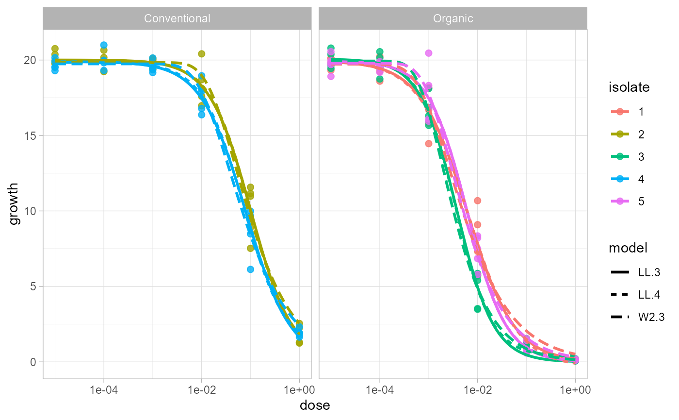
For a cleaner reporting figure, plot only the best-supported model in each isolate and stratum.
plot_EC50_curves(fit, models = "best")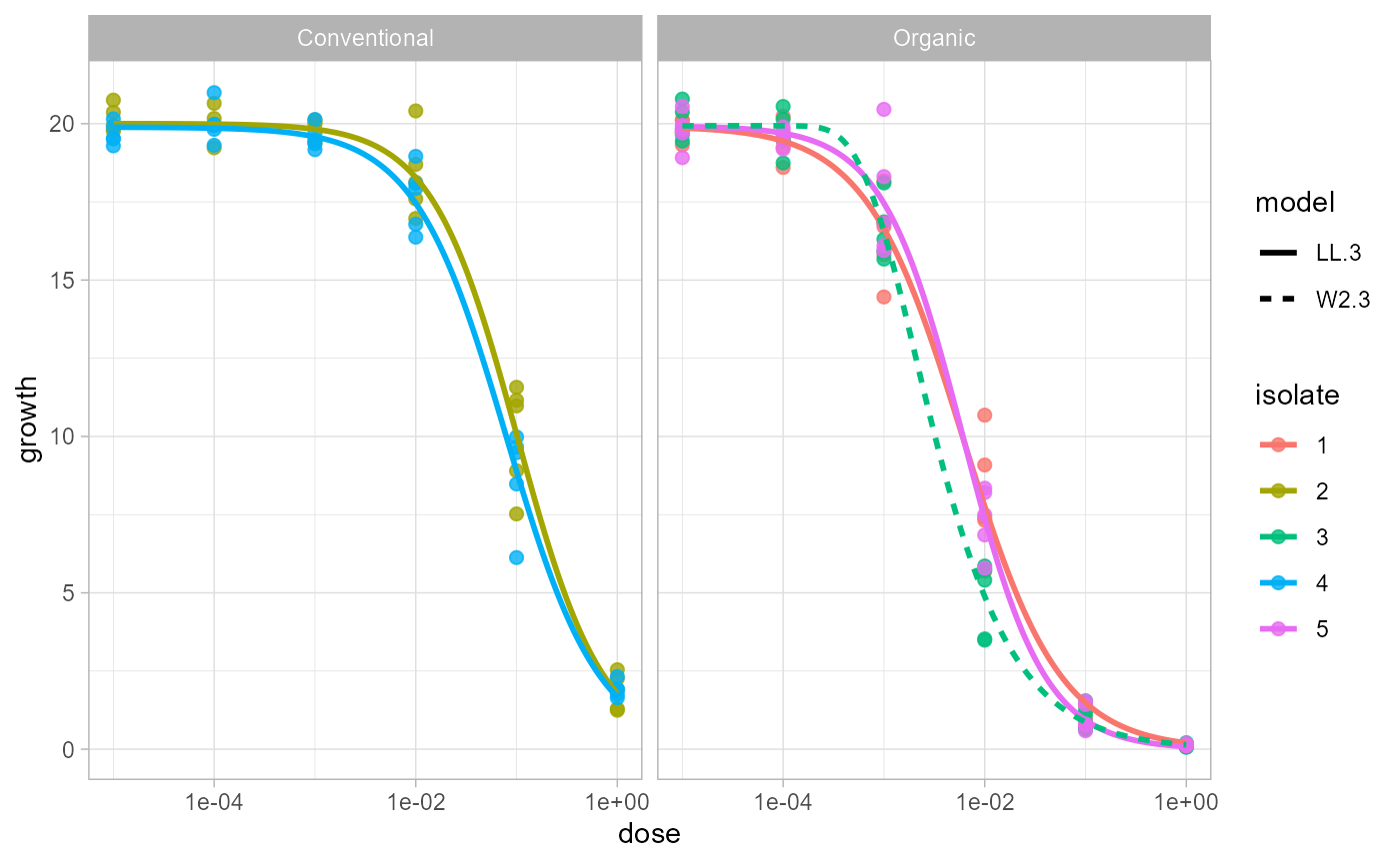
Customize with Curve Data
Use curve_data() when you want to build a custom
ggplot2 figure. This helper uses the stored models and does
not refit them.
curves <- curve_data(fit)

head(curves)
## field isolate model dose growth .curve_group
## 1 Organic 1 LL.3 1.000000e-05 19.86338 Organic.1.LL.3
## 1.1 Organic 1 LL.3 1.059560e-05 19.86006 Organic.1.LL.3
## 1.2 Organic 1 LL.3 1.122668e-05 19.85657 Organic.1.LL.3
## 1.3 Organic 1 LL.3 1.189534e-05 19.85289 Organic.1.LL.3
## 1.4 Organic 1 LL.3 1.260383e-05 19.84901 Organic.1.LL.3
## 1.5 Organic 1 LL.3 1.335452e-05 19.84493 Organic.1.LL.3
ggplot(curves, aes(dose, growth, color = factor(isolate), linetype = model)) +
  geom_line(linewidth = 1) +
  facet_wrap(~field) +
  scale_x_log10() +
  labs(x = "Dose", y = "Growth", color = "Isolate") +
  theme_light()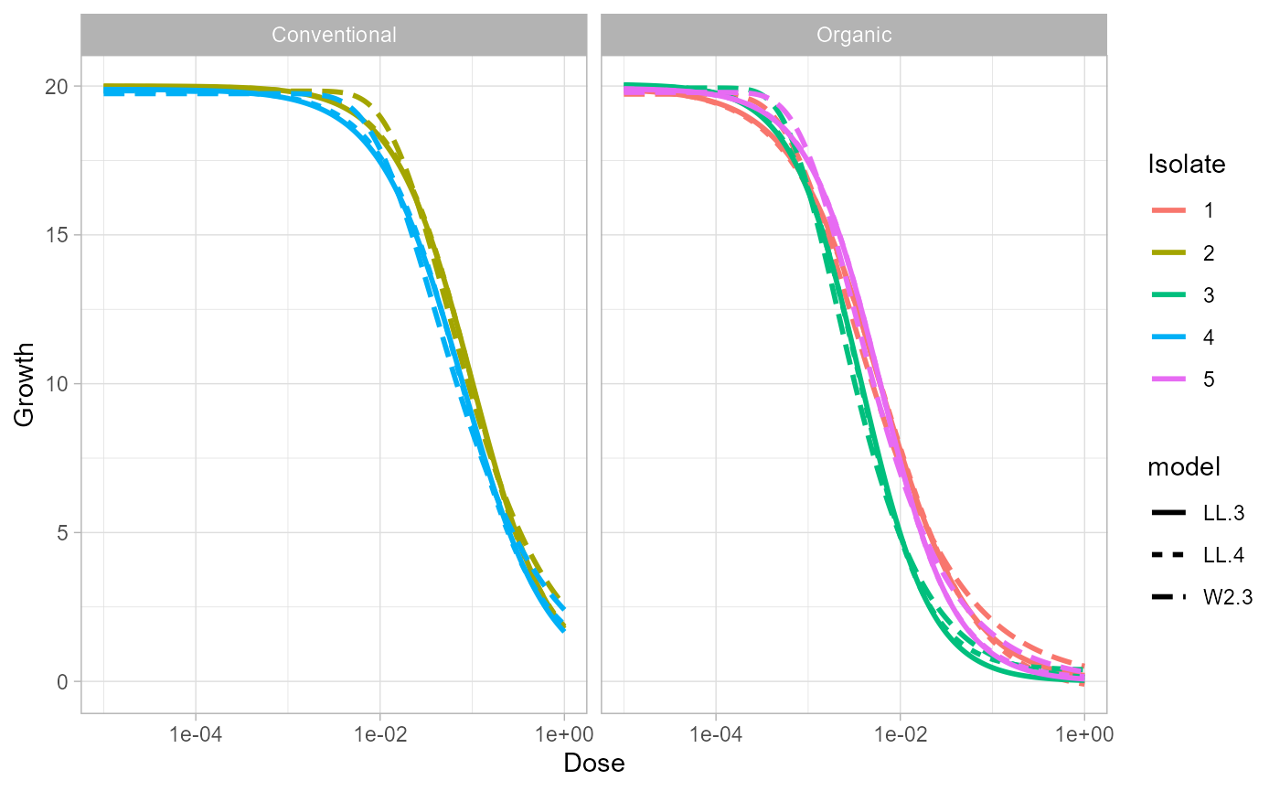
Predict and Report Selected Models
Use models = "best" when you want predictions or tables
from only the best-supported model in each group.
predict_ec50(
  fit,
  dose = c(0.001, 0.01, 0.1),
  models = "best"
)
## ID field model dose predicted
## 1 1 Organic LL.3 0.001 16.6397063
## 2 1 Organic LL.3 0.010 7.7646682
## 3 1 Organic LL.3 0.100 1.4846233
## 4 2 Conventional LL.3 0.001 19.8239563
## 5 2 Conventional LL.3 0.010 18.2773750
## 6 2 Conventional LL.3 0.100 10.0752898
## 7 4 Conventional LL.3 0.001 19.5825722
## 8 4 Conventional LL.3 0.010 17.4554970
## 9 4 Conventional LL.3 0.100 8.8966200
## 10 5 Organic LL.3 0.001 17.4586665
## 11 5 Organic LL.3 0.010 7.3837621
## 12 5 Organic LL.3 0.100 0.9303844
## 13 3 Organic W2.3 0.001 16.5443281
## 14 3 Organic W2.3 0.010 4.8836421
## 15 3 Organic W2.3 0.100 0.8690447
report_ec50(fit, models = "best")## ID field Estimate Std..Error Lower Upper logLik
## 1 1 Organic 0.006072082 0.0005740341 0.004902813 0.007241351 -45.15079
## 2 2 Conventional 0.101455765 0.0076364691 0.085900787 0.117010744 -43.53183
## 4 4 Conventional 0.079971237 0.0055655891 0.068634503 0.091307971 -38.42154
## 5 5 Organic 0.006122508 0.0004575060 0.005190599 0.007054418 -41.41058
## 13 3 Organic 0.003233688 0.0001397399 0.002949048 0.003518329 -34.48387
## IC Lack.of.fit Res.var model
## 1 98.30158 0.7271292 0.8451681 LL.3
## 2 95.06365 0.9866424 0.7704874 LL.3
## 4 84.84309 0.8328859 0.5753664 LL.3
## 5 90.82115 0.9744433 0.6825317 LL.3
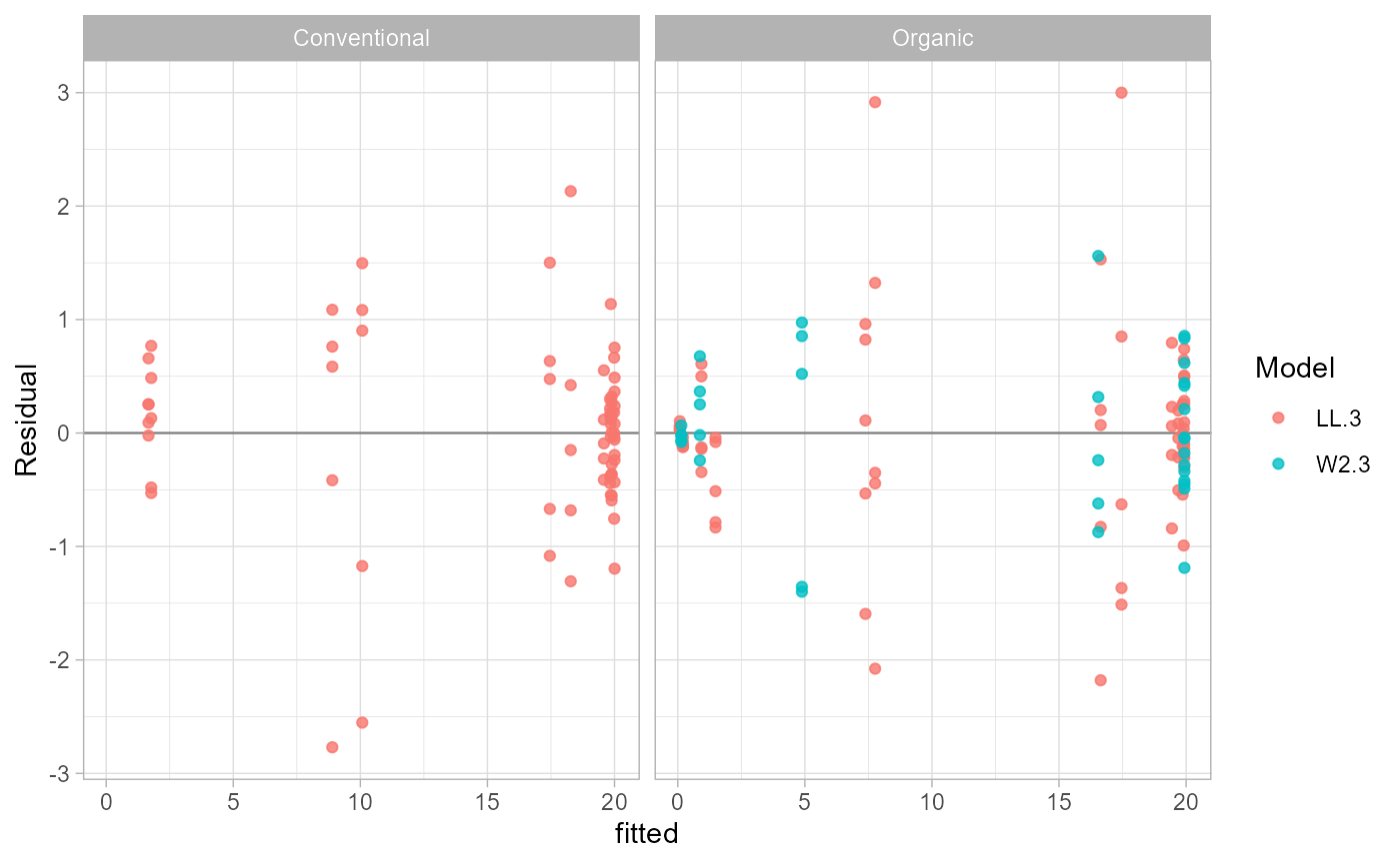
## 13 76.96774 0.8355451 0.4594349 W2.3Residual Diagnostics
Residuals can be returned as data or plotted with
ggplot2.
head(residual_data(fit, models = "best"))## ID field model dose observed fitted residual
## 1 1 Organic LL.3 0e+00 20.2082399 19.925747 0.2824926
## 2 1 Organic LL.3 1e-05 20.1168279 19.863383 0.2534450
## 3 1 Organic LL.3 1e-04 19.2479678 19.441644 -0.1936758
## 4 1 Organic LL.3 1e-03 15.8123455 16.639706 -0.8273608
## 5 1 Organic LL.3 1e-02 7.3206757 7.764668 -0.4439924
## 6 1 Organic LL.3 1e-01 0.6985264 1.484623 -0.7860970
plot_residuals(fit, models = "best")