Summarizing multivariable disease-favorable conditions

Many plant disease processes depend on combinations of weather variables. Temperature alone may not be enough, and humidity alone may not be enough, but warm and humid periods together can represent biologically favorable exposure. The .conditions entry in statistics lets a user summarize those multivariable rules inside each candidate window.

library(windcut)
library(dplyr)
library(ggplot2)
library(tidyr)
library(cowplot)

Function glossary

These functions are used inside the special .conditions entry of statistics. Each condition function receives the whole weather window, so the expression can combine temperature, humidity, rain, wetness, or any other columns in the weather table.

Function	What it does	Typical use
count_when()	Count rows where a multivariable condition is TRUE	Number of favorable observations
proportion_when()	Return the fraction of valid rows where the condition is TRUE	Compare favorable exposure across windows
sum_when()	Sum one variable only when the condition is TRUE	Rainfall during warm periods
mean_when()	Average one variable only when the condition is TRUE	Mean humidity during warm periods
max_when() / min_when()	Return the maximum or minimum of one variable when the condition is TRUE	Extremes during biologically favorable periods
max_consecutive_when()	Find the longest uninterrupted run where the condition is TRUE	Longest favorable spell
spell_count_when()	Count separate uninterrupted runs where the condition is TRUE	Number of favorable episodes
mean_spell_duration_when()	Average the length of favorable spells	Typical spell duration
max_spell_duration_when()	Return the length of the longest favorable spell	Maximum continuous exposure

Load weather and disease data

The condition expressions refer to the actual column names in the weather table. In this demo, the daily columns are named daily_mean_temp, daily_mean_rh, daily_sum_rain, and daily_sum_leaf_wetness.

data(window_pane_demo_data)

weather <- window_pane_demo_data$weather
assessments <- window_pane_demo_data$assessments

knitr::kable(head(weather))

site_id	date	time	daily_mean_temp	daily_mean_rh	daily_sum_rain	daily_sum_leaf_wetness
S01	2023-12-01	2023-12-01	22.33292	80.61750	7.15	6
S01	2023-12-02	2023-12-02	22.67500	78.64167	0.85	4
S01	2023-12-03	2023-12-03	23.35333	79.42042	3.61	7
S01	2023-12-04	2023-12-04	23.39167	77.86875	0.00	3
S01	2023-12-05	2023-12-05	23.13667	78.99000	6.59	6
S01	2023-12-06	2023-12-06	22.63375	80.20750	0.86	6

Make one condition visible

Before using .conditions, it helps to draw the rule on the time series. Here a day is called favorable when temperature is between 18 and 26 degrees C and relative humidity is at least 85%. The orange points are the observations that satisfy the full rule. The threshold is chosen to make the demo visible; a real analysis should use thresholds justified by the pathosystem.

example_site <- assessments$site_id[1]
example_reference <- assessments %>%
  filter(site_id == example_site) %>%
  pull(assessment_time)

condition_weather <- weather %>%
  filter(site_id == example_site) %>%
  filter(time >= example_reference - 35 * 86400, time <= example_reference) %>%
  mutate(
    favorable = daily_mean_temp >= 18 &
      daily_mean_temp <= 26 &
      daily_mean_rh >= 85,
    wet_and_warm = daily_sum_leaf_wetness > 0 &
      daily_mean_temp >= 18 &
      daily_mean_temp <= 26
  )

ggplot(condition_weather, aes(time, daily_mean_temp)) +
  geom_vline(
    xintercept = example_reference,
    linetype = "dashed",
    color = "#20262e",
    linewidth = 0.7
  ) +
  geom_ribbon(aes(ymin = 18, ymax = 26), fill = "#6ea87d", alpha = 0.12) +
  geom_line(color = "#20262e", linewidth = 0.8) +
  geom_point(
    data = condition_weather %>% filter(favorable),
    color = "#c47f2c",
    size = 2.6
  ) +
  labs(
    title = "A multivariable condition is a biological rule applied row by row",
    subtitle = "Orange points satisfy temperature and humidity requirements",
    x = NULL,
    y = "Daily mean temperature (deg C)"
  ) +
  theme_half_open()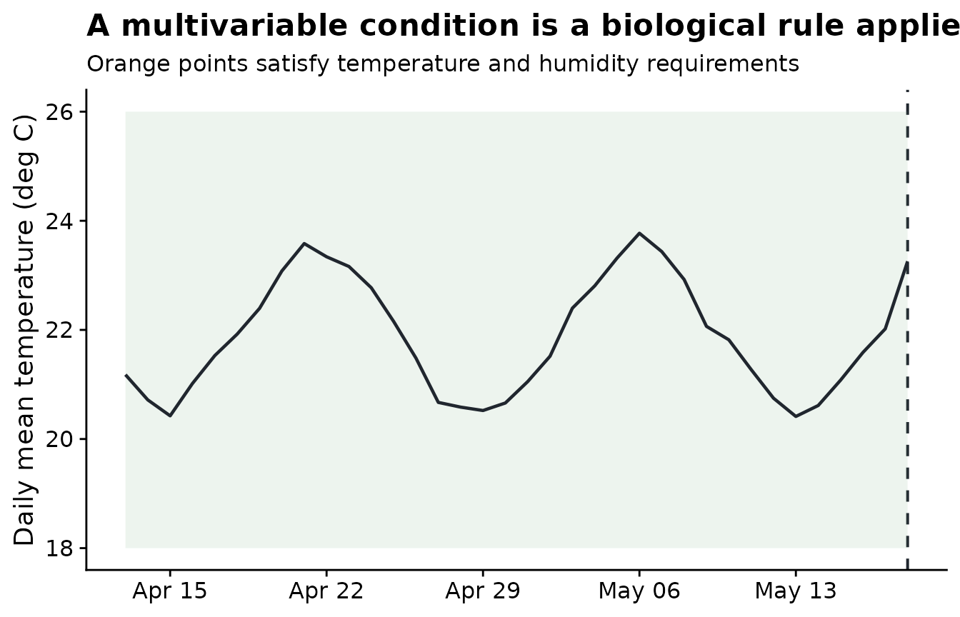

The same rule can be shown as a calendar-like condition timeline. This is often the easiest plot for checking whether the condition creates isolated favorable days or longer spells.

condition_timeline <- condition_weather %>%
  select(time, favorable, wet_and_warm) %>%
  pivot_longer(
    cols = c(favorable, wet_and_warm),
    names_to = "condition",
    values_to = "present"
  )

ggplot(condition_timeline, aes(time, condition, fill = present)) +
  geom_tile(color = "white", linewidth = 0.5, height = 0.8) +
  scale_fill_manual(values = c("FALSE" = "#e8ecef", "TRUE" = "#2b6c4f")) +
  labs(
    title = "Condition timelines reveal duration and interruption",
    x = NULL,
    y = NULL,
    fill = "Condition met"
  ) +
  theme_half_open() +
  theme(panel.grid = element_blank())

Define multivariable summaries

A condition summary receives the whole weather window as a data frame. That is why expressions can combine several variables. Output names from .conditions are not prefixed by one weather-variable name because the condition already describes a multivariable process.

summary_statistics <- list(
  daily_mean_temp = list(
    mean = "mean",
    days_18_26 = count_between(18, 26)
  ),
  daily_mean_rh = list(
    mean = "mean",
    humid_days = humid_hours(85)
  ),
  daily_sum_rain = list(
    total = "sum"
  ),
  daily_sum_leaf_wetness = list(
    wet_days = wet_days(0)
  ),
  .conditions = list(
    favorable_days = count_when(
      daily_mean_temp >= 18 & daily_mean_temp <= 26 & daily_mean_rh >= 85
    ),
    favorable_spell = max_consecutive_when(
      daily_sum_leaf_wetness > 0 & daily_mean_temp >= 18 & daily_mean_temp <= 26
    ),
    warm_rain_total = sum_when(
      daily_sum_rain,
      daily_mean_temp >= 18 & daily_mean_temp <= 28
    )
  )
)

Apply the rules inside candidate windows

The window-pane workflow does not change. The only difference is that statistics now includes .conditions.

windows <- make_windows(
  min_offset = -35,
  max_offset = 0,
  width = 7,
  slide_by = 7,
  reference_col = "assessment_time"
)

features <- window_pane(
  weather = weather,
  assessments = assessments,
  windows = windows,
  reference_col = "assessment_time",
  id_col = "site_id",
  response_col = "disease_intensity",
  unit = "days",
  statistics = summary_statistics
)

features %>%
  select(site_id, disease_intensity, contains("favorable"), contains("warm_rain")) %>%
  slice_head(n = 6) %>%
  knitr::kable()

site_id	disease_intensity	favorable_days_window_m35_m28	favorable_spell_window_m35_m28	favorable_days_window_m28_m21	favorable_spell_window_m28_m21	favorable_days_window_m21_m14	favorable_spell_window_m21_m14	favorable_days_window_m14_m07	favorable_spell_window_m14_m07	favorable_days_window_m07_z00	favorable_spell_window_m07_z00	warm_rain_total_window_m35_m28	warm_rain_total_window_m28_m21	warm_rain_total_window_m21_m14	warm_rain_total_window_m14_m07	warm_rain_total_window_m07_z00
S01	75.2	0	7	0	7	0	7	0	7	0	7	24.15	26.60	24.41	2.97	20.31
S02	59.2	0	7	0	7	0	7	0	7	0	7	5.51	24.52	22.33	24.98	45.46
S03	53.9	0	7	0	7	0	7	0	7	0	7	17.59	21.36	34.21	19.35	17.91
S04	71.7	0	7	0	7	0	7	0	7	0	7	23.45	16.45	9.04	8.94	20.53
S05	80.9	0	7	0	7	0	7	0	7	0	7	9.45	26.14	12.47	12.88	9.37
S06	87.2	0	7	0	7	0	7	0	7	0	7	29.88	21.78	17.80	14.52	18.87

Compare condition functions in the output

favorable_days counts how many rows inside a window satisfy the full temperature-humidity rule. favorable_spell measures the longest uninterrupted wet-and-warm period. warm_rain_total sums rain only on rows where temperature is inside the selected range.

This article stops at interpretation of the generated variables. It does not try to demonstrate a disease-response relationship, because that belongs in a later screening or modeling workflow.

condition_examples <- features |>
  select(site_id, contains("favorable"), contains("warm_rain")) |>
  slice_head(n = 6)

knitr::kable(condition_examples)

site_id	favorable_days_window_m35_m28	favorable_spell_window_m35_m28	favorable_days_window_m28_m21	favorable_spell_window_m28_m21	favorable_days_window_m21_m14	favorable_spell_window_m21_m14	favorable_days_window_m14_m07	favorable_spell_window_m14_m07	favorable_days_window_m07_z00	favorable_spell_window_m07_z00	warm_rain_total_window_m35_m28	warm_rain_total_window_m28_m21	warm_rain_total_window_m21_m14	warm_rain_total_window_m14_m07	warm_rain_total_window_m07_z00
S01	0	7	0	7	0	7	0	7	0	7	24.15	26.60	24.41	2.97	20.31
S02	0	7	0	7	0	7	0	7	0	7	5.51	24.52	22.33	24.98	45.46
S03	0	7	0	7	0	7	0	7	0	7	17.59	21.36	34.21	19.35	17.91
S04	0	7	0	7	0	7	0	7	0	7	23.45	16.45	9.04	8.94	20.53
S05	0	7	0	7	0	7	0	7	0	7	9.45	26.14	12.47	12.88	9.37
S06	0	7	0	7	0	7	0	7	0	7	29.88	21.78	17.80	14.52	18.87

The plot below uses one site to show how the condition summaries differ across candidate windows. The bars are not a model result; they are a check that each condition function produced the intended biological quantity.

condition_features <- features |>
  filter(site_id == example_site) |>
  select(contains("favorable_days"), contains("favorable_spell"), contains("warm_rain_total")) |>
  pivot_longer(
    cols = everything(),
    names_to = "feature",
    values_to = "value"
  ) |>
  mutate(
    window = sub(".*_window_", "window_", feature),
    summary_class = case_when(
      grepl("favorable_days", feature) ~ "Count of favorable days",
      grepl("favorable_spell", feature) ~ "Longest favorable spell",
      grepl("warm_rain_total", feature) ~ "Rain during warm days",
      TRUE ~ "Condition summary"
    ),
    window = factor(window, levels = unique(window))
  )

ggplot(condition_features, aes(window, value, fill = summary_class)) +
  geom_col(show.legend = FALSE) +
  facet_wrap(~ summary_class, scales = "free_y", ncol = 1) +
  labs(
    title = "Condition functions summarize different biological quantities",
    subtitle = "Example values for one site across 7-day candidate windows",
    x = "Candidate window",
    y = "Summary value"
  ) +
  theme_half_open() +
  theme(axis.text.x = element_text(angle = 35, hjust = 1))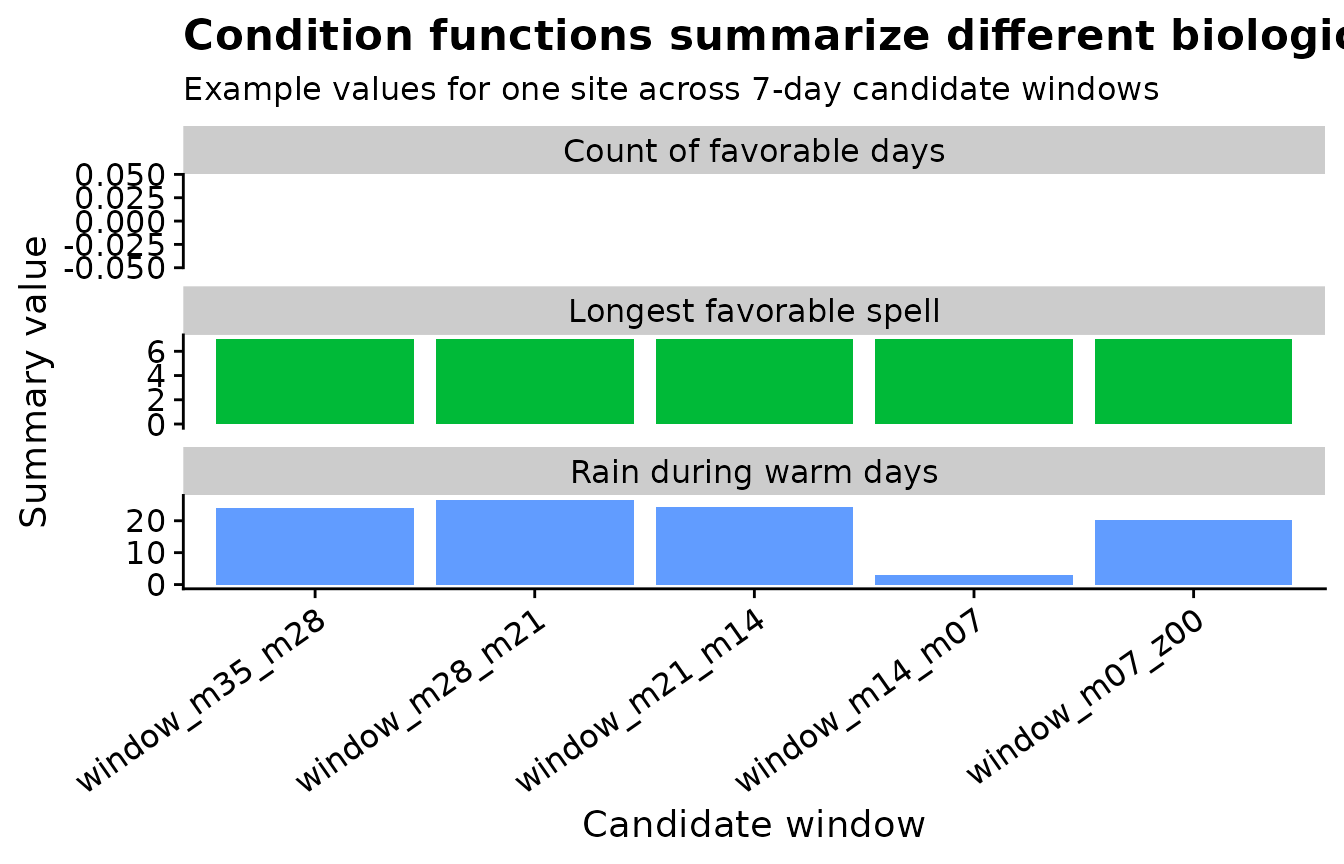

Use .conditions when the biological rule depends on more than one weather variable. Use variable-specific summaries when the statistic only needs one column, such as mean temperature, total rain, or humid observations.