Deriving biologically meaningful weather summaries • windcut

This article shows how to turn weather records into predictors that are easier to interpret biologically. A mean temperature can be useful, but plant disease risk often depends on exposure: how many observations were warm enough, how long humidity stayed high, whether rain occurred as an event, or how much thermal time accumulated inside a candidate window.

library(windcut)
library(dplyr)
library(ggplot2)
library(tidyr)
library(cowplot)

Function glossary

These functions can be placed inside statistics to create biologically interpretable summaries from one weather variable at a time.

Function	What it does	Typical use
`count_above()` / `count_at_or_above()`	Count observations above a threshold	Hot, humid, rainy, or wet observations
`count_between()`	Count observations inside a biological range	Days with temperature between lower and upper limits
`proportion_above()` / `proportion_between()`	Return the fraction of valid observations meeting a rule	Compare exposure across windows with different numbers of records
`sum_above()` / `sum_between()`	Sum values only when a threshold rule is met	Rain amount during selected conditions
`mean_above()` / `mean_between()`	Average values only when a threshold rule is met	Mean temperature during favorable periods
`degree_hours_above()` / `degree_days_above()`	Accumulate thermal time above a base value	Temperature-driven development
`humid_hours()` / `proportion_humid()`	Count or quantify high-humidity observations	Humidity exposure
`rainy_hours()` / `rain_events()`	Count rainy observations or consecutive rain events	Event-driven rainfall exposure
`wet_hours()` / `wet_days()`	Count wet observations	Leaf-wetness duration
`max_consecutive_wet_hours()`	Find the longest uninterrupted wet period	Continuous infection-favorable wetness
`derive_vpd()` / `derive_dew_point()`	Add derived humidity variables to the weather table	Atmospheric dryness and dew-point interpretation
`derive_leaf_wetness_from_rh()`	Estimate wetness from high relative humidity	Projects without measured leaf wetness

Start from daily weather

The bundled demo data contain one daily weather series per site and one disease assessment per site. This article starts from daily data so the focus stays on the biological summaries rather than on raw-data preparation.

data(window_pane_demo_data)

weather <- window_pane_demo_data$weather
assessments <- window_pane_demo_data$assessments

knitr::kable(head(weather))

site_id	date	time	daily_mean_temp	daily_mean_rh	daily_sum_rain	daily_sum_leaf_wetness
S01	2023-12-01	2023-12-01	22.33292	80.61750	7.15	6
S01	2023-12-02	2023-12-02	22.67500	78.64167	0.85	4
S01	2023-12-03	2023-12-03	23.35333	79.42042	3.61	7
S01	2023-12-04	2023-12-04	23.39167	77.86875	0.00	3
S01	2023-12-05	2023-12-05	23.13667	78.99000	6.59	6
S01	2023-12-06	2023-12-06	22.63375	80.20750	0.86	6

Derive variables before summarizing

Some epidemiological predictors are not measured directly. For example, vapor pressure deficit is derived from temperature and relative humidity, and leaf wetness can be approximated from high relative humidity when measured wetness is not available. windcut keeps this step explicit: the original weather table is returned with new columns.

weather <- weather |>
  derive_vpd(daily_mean_temp, daily_mean_rh, name = "daily_vpd") |>
  derive_leaf_wetness_from_rh(
    daily_mean_rh,
    threshold = 85,
    name = "daily_leaf_wetness_est"
  )

weather |>
  select(site_id, time, daily_mean_temp, daily_mean_rh, daily_vpd, daily_leaf_wetness_est) |>
  slice_head(n = 8) |>
  knitr::kable()

site_id	time	daily_mean_temp	daily_mean_rh	daily_vpd
S01	2023-12-01	22.33292	80.61750	0.5229513
S01	2023-12-02	22.67500	78.64167	0.5883544
S01	2023-12-03	23.35333	79.42042	0.5906425
S01	2023-12-04	23.39167	77.86875	0.6366462
S01	2023-12-05	23.13667	78.99000	0.5951597
S01	2023-12-06	22.63375	80.20750	0.5438584
S01	2023-12-07	22.24750	79.78875	0.5424861
S01	2023-12-08	21.59917	80.14833	0.5121772

The plot below shows why this is useful. The derived variables make the biological interpretation visible before any modeling: high humidity creates estimated wetness, and lower VPD indicates more humid atmospheric conditions. The 85% relative-humidity threshold is used here only to make the example easy to see; a real analysis should use a biologically justified threshold.

example_site <- assessments$site_id[1]
example_reference <- assessments %>%
  filter(site_id == example_site) %>%
  pull(assessment_time)

derived_plot_data <- weather %>%
  filter(site_id == example_site) %>%
  filter(time >= example_reference - 35 * 86400, time <= example_reference) %>%
  select(time, daily_mean_rh, daily_vpd, daily_leaf_wetness_est) %>%
  pivot_longer(
    cols = c(daily_mean_rh, daily_vpd, daily_leaf_wetness_est),
    names_to = "variable",
    values_to = "value"
  )

ggplot(derived_plot_data, aes(time, value)) +
  geom_vline(
    xintercept = example_reference,
    linetype = "dashed",
    color = "#20262e",
    linewidth = 0.7
  ) +
  geom_line(color = "#3f7d58", linewidth = 0.8) +
  facet_wrap(~ variable, scales = "free_y", ncol = 1) +
  labs(
    title = "Derived variables make the weather signal easier to inspect",
    subtitle = "The dashed line marks the disease assessment date",
    x = NULL,
    y = NULL
  ) +
  theme_half_open()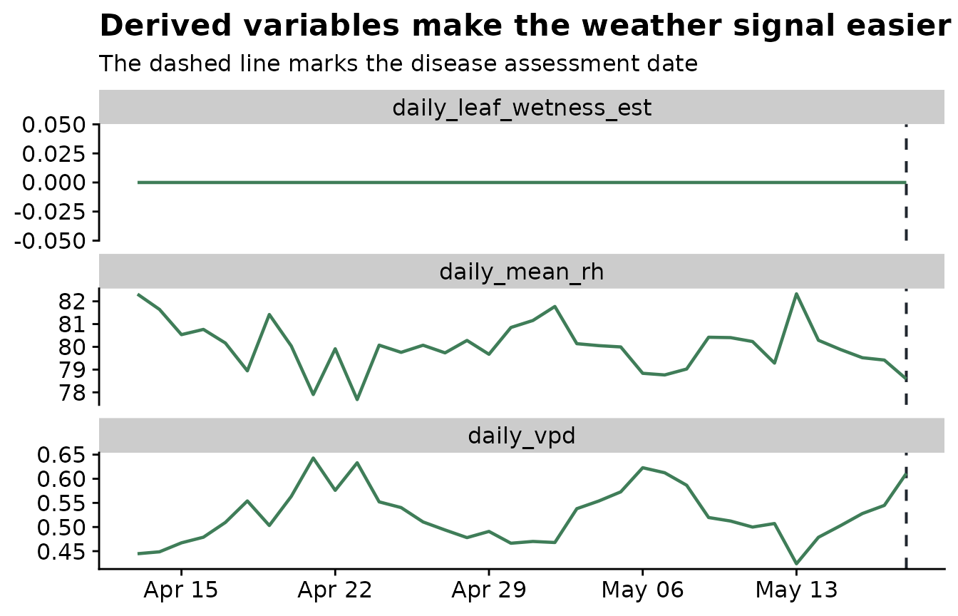

ggplot2 chart showing biologically meaningful weather summaries.

Translate biological ideas into summaries

Each summary function returns a function that can be used inside statistics. The names you choose on the left become part of the output feature names. This makes the resulting columns readable: daily_mean_rh_humid_days is easier to interpret than an anonymous transformed value.

summary_statistics <- list(
  daily_mean_temp = list(
    mean = "mean",
    days_18_26 = count_between(18, 26),
    thermal_time_10 = degree_hours_above(10)
  ),
  daily_mean_rh = list(
    mean = "mean",
    humid_days = humid_hours(85),
    prop_humid = proportion_at_or_above(85)
  ),
  daily_vpd = list(
    mean = "mean",
    dry_days = count_above(1.2)
  ),
  daily_sum_rain = list(
    total = "sum",
    rainy_days = rainy_days(0),
    rain_events = rain_events(0.2)
  ),
  daily_leaf_wetness_est = list(
    wet_days = wet_days(0),
    max_wet_spell = max_consecutive_wet_hours(0)
  )
)

The next plot shows several of those biological rules on one site. Warm days are observations inside the 18 to 26 degree C range. Humid days have relative humidity at or above 85%. Wet days are derived from relative humidity.

rule_plot_data <- weather %>%
  filter(site_id == example_site) %>%
  filter(time >= example_reference - 35 * 86400, time <= example_reference) %>%
  mutate(
    warm_18_26 = daily_mean_temp >= 18 & daily_mean_temp <= 26,
    humid = daily_mean_rh >= 85,
    wet_estimated = daily_leaf_wetness_est > 0
  )

ggplot(rule_plot_data, aes(time, daily_mean_temp)) +
  geom_vline(
    xintercept = example_reference,
    linetype = "dashed",
    color = "#20262e",
    linewidth = 0.7
  ) +
  geom_ribbon(
    aes(ymin = 18, ymax = 26),
    fill = "#6ea87d",
    alpha = 0.12
  ) +
  geom_line(color = "#20262e", linewidth = 0.8) +
  geom_point(
    data = rule_plot_data %>% filter(warm_18_26 & humid),
    color = "#c47f2c",
    size = 2.4
  ) +
  geom_point(
    data = rule_plot_data %>% filter(wet_estimated),
    aes(y = 17),
    color = "#2b6c4f",
    size = 2,
    alpha = 0.85
  ) +
  labs(
    title = "Biological rules can be inspected before feature generation",
    subtitle = "Orange points are warm-and-humid days; green points along the bottom are estimated wet days",
    x = NULL,
    y = "Daily mean temperature (deg C)"
  ) +
  theme_half_open()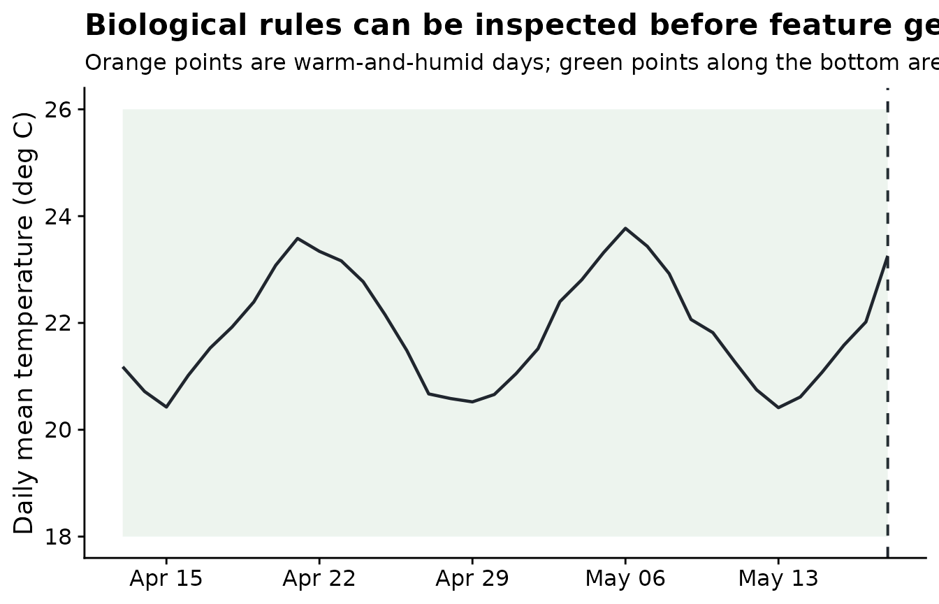

ggplot2 chart showing biologically meaningful weather summaries.

Summarize inside candidate windows

Now the biological summaries are applied inside 7-day candidate windows ending at the assessment date. The result is one row per site and one feature column per summary-window combination.

windows <- make_windows(
  min_offset = -28,
  max_offset = 0,
  width = 7,
  slide_by = 7,
  reference_col = "assessment_time"
)

features <- window_pane(
  weather = weather,
  assessments = assessments,
  windows = windows,
  reference_col = "assessment_time",
  id_col = "site_id",
  response_col = "disease_intensity",
  unit = "days",
  statistics = summary_statistics
)

features %>%
  select(1:12) %>%
  slice_head(n = 6) %>%
  knitr::kable()

site_id	assessment_time	disease_intensity	n_obs_window_m28_m21	daily_mean_temp_mean_window_m28_m21	daily_mean_temp_days_18_26_window_m28_m21	daily_mean_temp_thermal_time_10_window_m28_m21	daily_mean_rh_mean_window_m28_m21	daily_vpd_mean_window_m28_m21
S01	2024-05-18	75.2	7	22.79661	7	89.57625	79.34881	0.5740978
S02	2024-05-07	59.2	7	21.73744	7	82.16208	80.51815	0.5099807
S03	2024-05-20	53.9	7	22.09607	7	84.67250	79.74393	0.5415874
S04	2024-04-12	71.7	7	21.06881	7	77.48167	80.37393	0.4902537
S05	2024-04-29	80.9	7	21.83857	7	82.87000	80.00417	0.5252337
S06	2024-04-15	87.2	7	21.74185	7	82.19292	80.41304	0.5115775

Compare function classes in the output

The final feature table is ordinary modeling data. Each column combines three pieces of information: the weather variable, the biological summary, and the relative-time window. At this stage, the goal is only to confirm that the functions created interpretable columns; screening and modeling can come later.

The table below selects one example from several function classes: a temperature range count, thermal accumulation, humidity exposure, rain events, and wet-spell duration.

example_columns <- features |>
  select(
    site_id,
    contains("daily_mean_temp_days_18_26"),
    contains("daily_mean_temp_thermal_time_10"),
    contains("daily_mean_rh_humid_days"),
    contains("daily_sum_rain_rain_events"),
    contains("daily_leaf_wetness_est_max_wet_spell")
  ) |>
  select(1:11)

example_columns |>
  slice_head(n = 5) |>
  knitr::kable()

site_id	daily_mean_temp_days_18_26_window_m28_m21	daily_mean_temp_days_18_26_window_m21_m14	daily_mean_temp_days_18_26_window_m14_m07	daily_mean_temp_days_18_26_window_m07_z00	daily_mean_temp_thermal_time_10_window_m28_m21	daily_mean_temp_thermal_time_10_window_m21_m14	daily_mean_temp_thermal_time_10_window_m14_m07	daily_mean_temp_thermal_time_10_window_m07_z00
S01	7	7	7	7	89.57625	77.40792	90.13833	77.73292
S02	7	7	7	7	82.16208	85.40125	81.48792	86.79583
S03	7	7	7	7	84.67250	82.00083	84.60875	82.62000
S04	7	7	7	7	77.48167	90.14833	77.92208	90.34417
S05	7	7	7	7	82.87000	85.96042	81.67333	86.11917

A compact plot is often easier to inspect than a very wide table. Here one site is used only as a worked example, and the facets separate the function classes.

class_plot_data <- features |>
  filter(site_id == example_site) |>
  select(
    contains("daily_mean_temp_days_18_26"),
    contains("daily_mean_rh_humid_days"),
    contains("daily_sum_rain_rain_events"),
    contains("daily_leaf_wetness_est_max_wet_spell")
  ) |>
  pivot_longer(
    cols = everything(),
    names_to = "feature",
    values_to = "value"
  ) |>
  mutate(
    window = sub(".*_window_", "window_", feature),
    summary_class = case_when(
      grepl("days_18_26", feature) ~ "Temperature range count",
      grepl("humid_days", feature) ~ "Humidity exposure",
      grepl("rain_events", feature) ~ "Rain events",
      grepl("max_wet_spell", feature) ~ "Wet-spell duration",
      TRUE ~ "Summary"
    ),
    window = factor(window, levels = unique(window))
  )

ggplot(class_plot_data, aes(window, value, fill = summary_class)) +
  geom_col(show.legend = FALSE) +
  facet_wrap(~ summary_class, scales = "free_y", ncol = 2) +
  labs(
    title = "Different function classes create different biological summaries",
    subtitle = "Example values for one site across 7-day candidate windows",
    x = "Candidate window",
    y = "Summary value"
  ) +
  theme_half_open() +
  theme(axis.text.x = element_text(angle = 35, hjust = 1))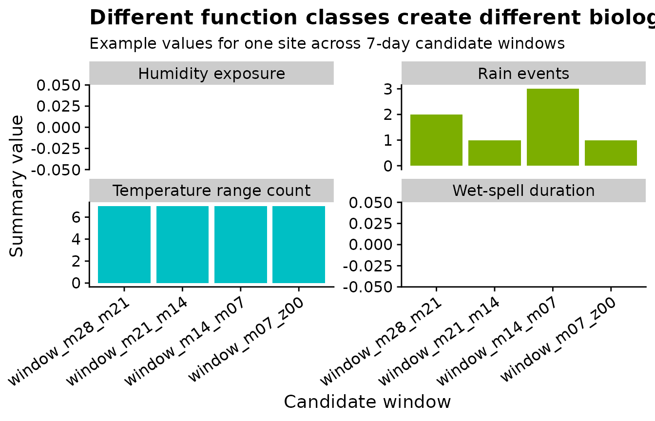

ggplot2 chart showing biologically meaningful weather summaries.

Recommended practices

Choose summaries that match the biology of the pathosystem. Use counts or proportions for threshold exposure, spell summaries for uninterrupted favorable periods, rain-event summaries for event-driven processes, and thermal-time summaries when accumulation above a base temperature is meaningful.