windcut helps plant disease epidemiologists convert weather time series into relative-time window features that can be used in forecasting and explanatory models of disease intensity.
Slice
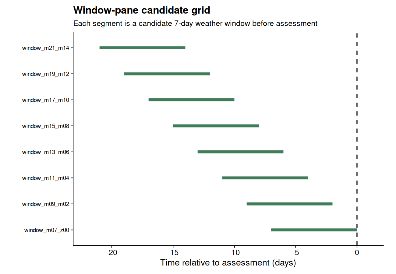
Generate many candidate windows relative to a user-chosen reference date using a window-pane strategy. Use fixed-width windows for a classic sliding scan, or variable-width windows when the exposure duration is uncertain.
Learning path
- Start with the Getting Started tutorial to understand the core workflow.
- Move to the window-pane tutorial to think like an epidemiologist when defining candidate periods.
- Use the feature-screening tutorial to prioritize windows before fitting predictive models.
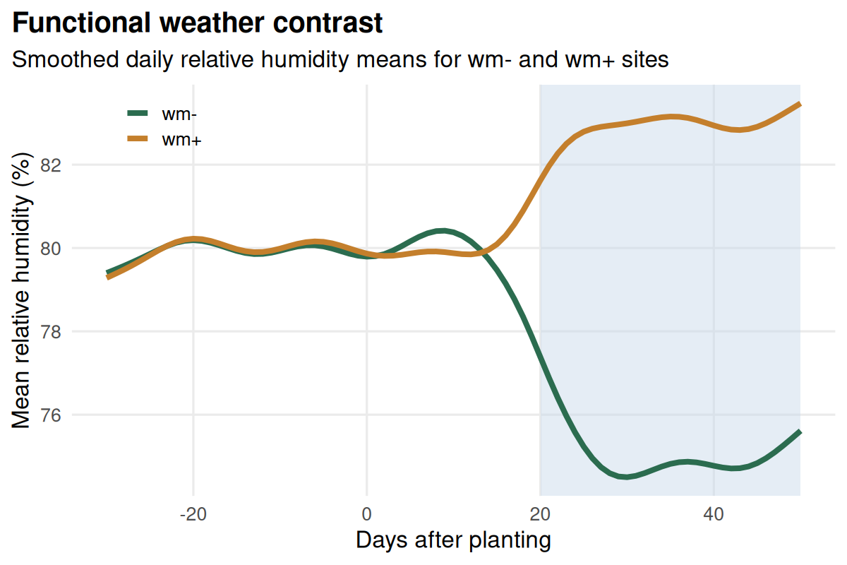
- Explore the FDA tutorial when you want to work with entire weather trajectories instead of pre-cut windows.
Quick start
The quick start uses the bundled demo dataset. It loads daily weather and one disease assessment per site, defines sliding weather windows, builds model-ready predictors, ranks features against the response, and identifies a less redundant predictor set for modeling.
library(windcut)

data(window_pane_demo_data)

weather <- window_pane_demo_data$weather
assessments <- window_pane_demo_data$assessments

windows <- make_windows(
  min_offset = -21,
  max_offset = 0,
  width = 7,
  reference_col = "assessment_time"
)

features <- window_pane(
  weather = weather,
  assessments = assessments,
  windows = windows,
  id_col = "site_id",
  response_col = "disease_intensity",
  statistics = list(
    daily_mean_temp = list(mean = "mean", days_18_26 = count_between(18, 26)),
    daily_mean_rh = list(mean = "mean", humid_days = humid_hours(90)),
    daily_sum_rain = list(total = "sum")
  )
)

screened <- screen_window_features(
  data = features,
  response_col = "disease_intensity",
  method = "spearman"
)

less_redundant <- screen_feature_correlations(
  data = features,
  exclude_cols = c("site_id", "assessment_time", "disease_intensity"),
  method = "spearman",
  threshold = 0.8
)
Core ideas
- Window-pane analysis is useful when the biologically relevant period is not known in advance.
- Weather summaries should stay interpretable enough to discuss with domain experts.
- Highly correlated predictors can be screened before modeling workflows that need less redundant inputs.
- Screening is only one step; the best windows still need validation in predictive models.