Data analysis

Packages

Here we load all the packages we ae going to use in the analysis.

library(tidyverse)
library(gsheet)
library(cowplot)
library(ggthemes)
library(DescTools)
library(minpack.lm)
library(agricolae)
library(readxl)
library(patchwork)

Probability distributions

Fist step is to assemble the probability distributions for the for variable we are going to use for the simulations

SBR severity on untreated check.

Import data

Importing data of soybean rust severity (SBR) on the untreated check

sev_data = read.csv("data/sev_data.csv")
head(sev_data)

Filtering only values of severity in the check treatment

sev_check = sev_data %>% 
  filter(active_ingredient == "check")
head(sev_check)

Empirical distribution

sev_check %>% 
  ggplot(aes(severity/100))+
  geom_histogram(bins = 20, color = "black", fill = "gray")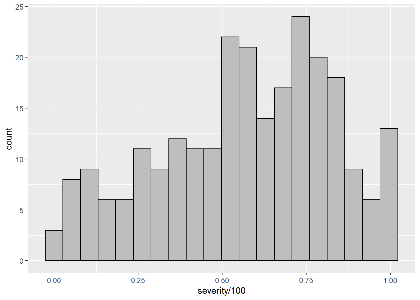

Modeling

Since severity in proportional terms is between zero and one, we fit the empirical distribution into a beta probability distribution. For that we need to find the shape and scale parameters of the beta distribution function.

For that, obtain the empirical cumulative distribution and fit to the beta cumulative distribution.

sev = sev_check$severity
Fx= environment(ecdf(sev))$y
x = environment(ecdf(sev))$x/100

summary(nlsLM(Fx ~ pbeta(x, shape1, shape2, log = FALSE) ,
      start = c(shape1 = 1, shape2 = 1),
      control = nls.lm.control(maxiter = 100000)))

## Warning in nls.lm(par = start, fn = FCT, jac = jac, control = control, lower =
## lower, : resetting `maxiter' to 1024!

## 
## Formula: Fx ~ pbeta(x, shape1, shape2, log = FALSE)
## 
## Parameters:
##        Estimate Std. Error t value Pr(>|t|)    
## shape1  1.70736    0.02761   61.83   <2e-16 ***
## shape2  1.26581    0.01925   65.75   <2e-16 ***
## ---
## Signif. codes:  0 '***' 0.001 '**' 0.01 '*' 0.05 '.' 0.1 ' ' 1
## 
## Residual standard error: 0.02053 on 186 degrees of freedom
## 
## Number of iterations to convergence: 6 
## Achieved convergence tolerance: 1.49e-08

Kolmogorov-Smirnov Test

ks.test(Fx,pbeta(x, 1.707, 1.266) )

## Warning in ks.test(Fx, pbeta(x, 1.707, 1.266)): p-value will be approximate in
## the presence of ties

## 
##  Two-sample Kolmogorov-Smirnov test
## 
## data:  Fx and pbeta(x, 1.707, 1.266)
## D = 0.053191, p-value = 0.953
## alternative hypothesis: two-sided

plot(x,Fx)
curve(pbeta(x, 1.707, 1.266),0,1, add = T)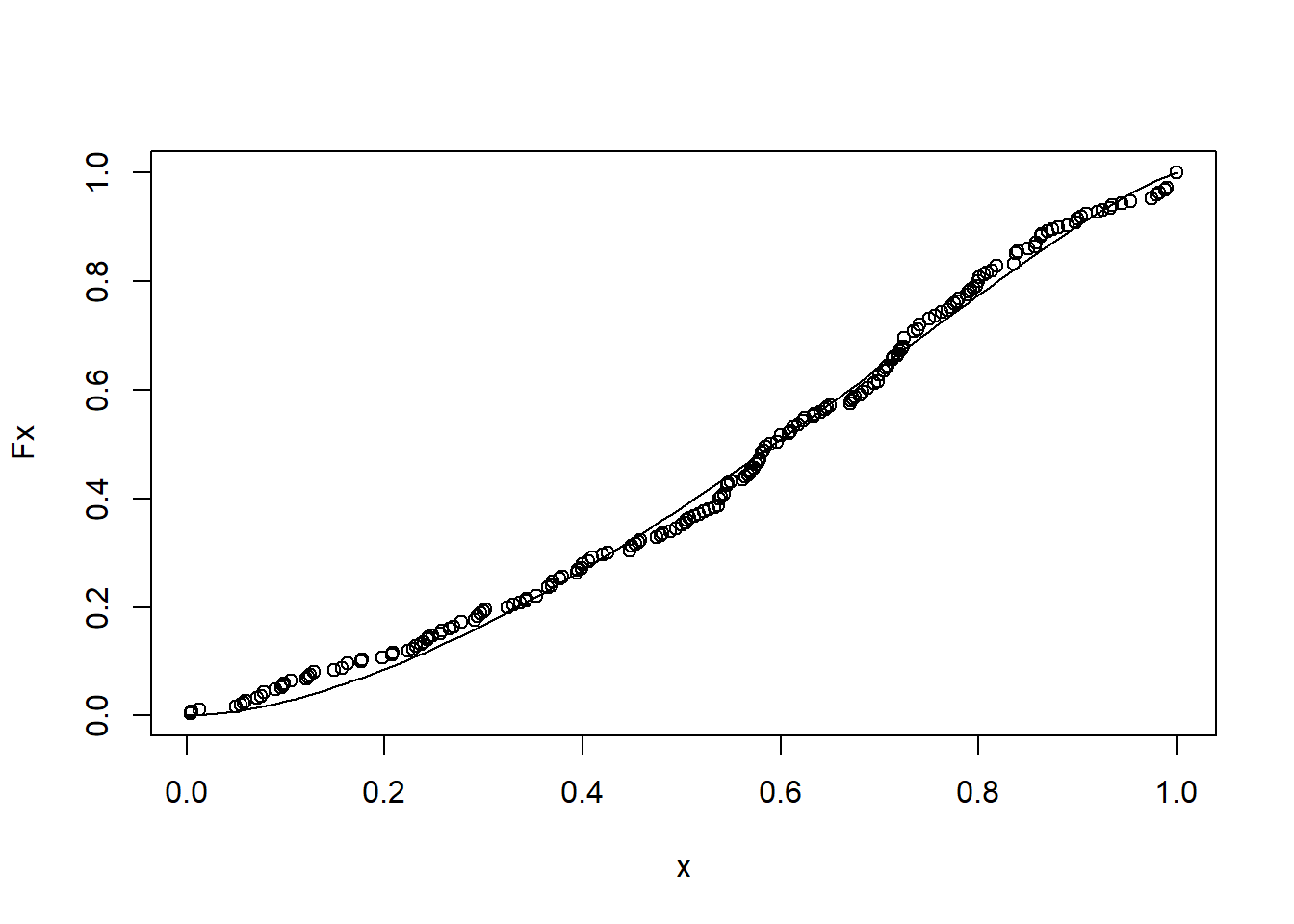

plot(Fx,pbeta(x, 1.707, 1.266) )
abline(a=0,b=1)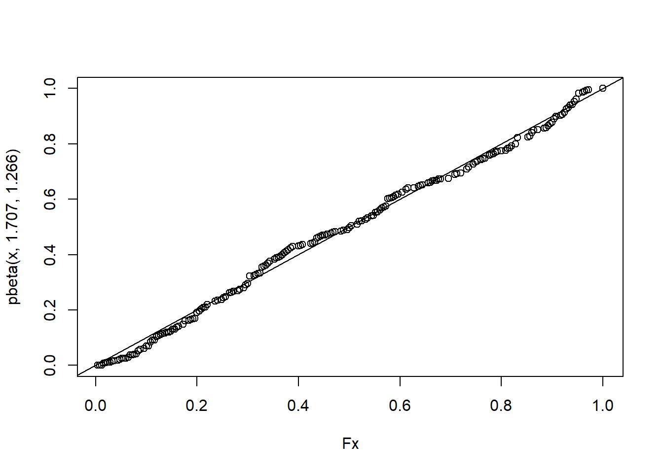

Visualization

sev_dist_plot = sev_check %>% 
  ggplot(aes(severity/100))+
 geom_histogram(aes(y = ..density..),bins = 10, color = "white", fill = "#AC08FF")+
   stat_function(fun=function(x) dbeta(x, 1.707, 1.266), color= "black", size = 1.2)+
  theme_bw()+
  labs(x="Severity (proportion)", y = "Density")
sev_dist_plot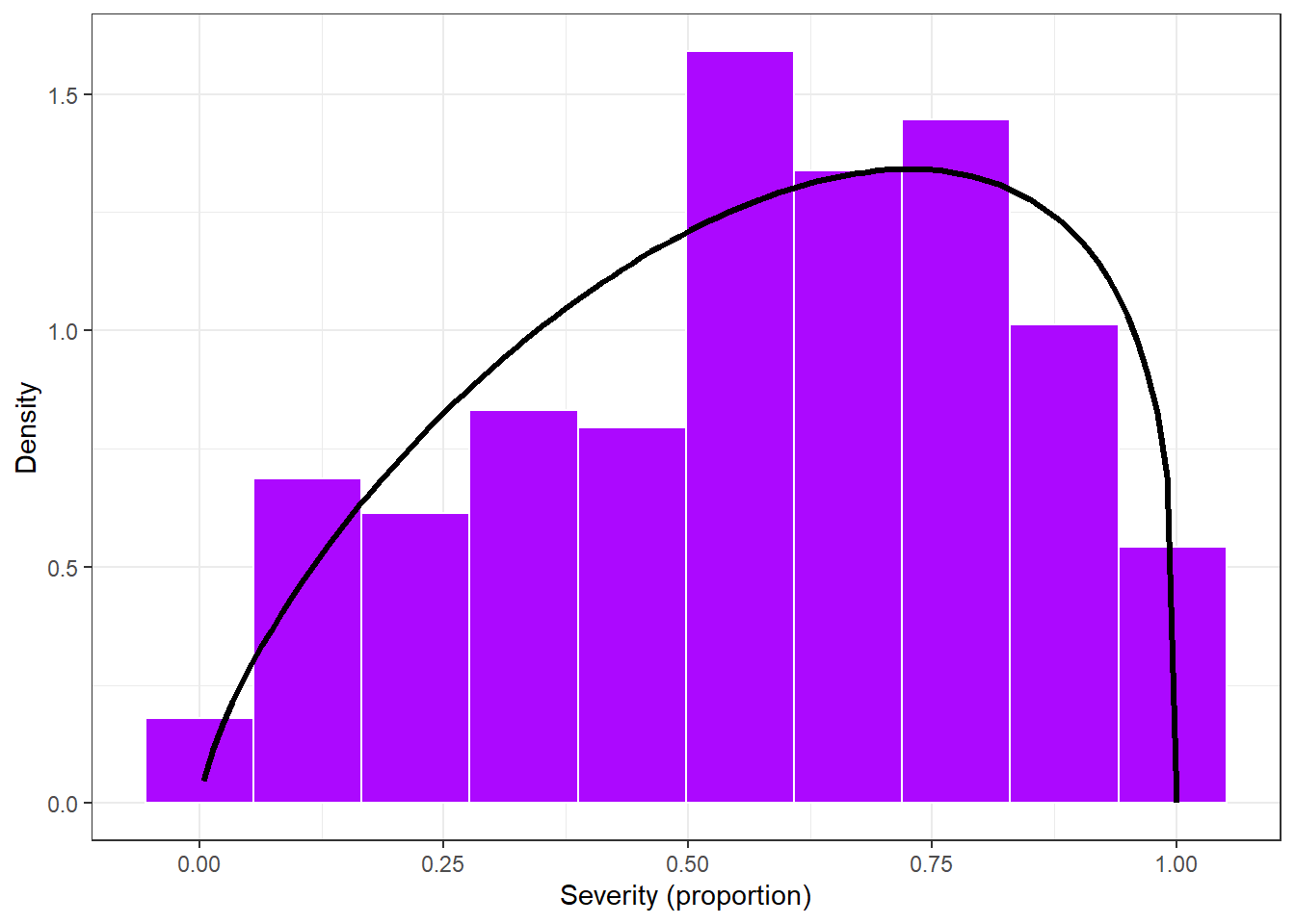

# ggsave("figs/sev_dist.png", dpi=600, height = 3, width = 4)

Soybean price

Import data

soybean = gsheet2tbl("https://docs.google.com/spreadsheets/d/1-jQ9OgWdLQCb0iB0FqbrhuVi7LiNhqxvf9QU4-iuc3o/edit#gid=1085329359") 
head(soybean)

conversion to US dollar

sbr_price = soybean %>% 
  filter(year>=2018) %>% 
  mutate(price = (price/60)/4,
         national_price = (national_price/60)/4)
sbr_price

sbr_price %>% 
  ggplot(aes(year,price)) +
  geom_jitter(alpha =.2, size =2)+
  geom_boxplot(aes(group = year), fill = NA, size= 1)+
  scale_color_gradient()+
  theme_minimal_hgrid()

  # facet_wrap(~state)

Mean and Standad deviantion

mean(sbr_price$price)

## [1] 0.2932792

sd(sbr_price$price)

## [1] 0.02167031

Empirical distribution

sbr_price %>% 
  ggplot(aes(price))+
  geom_histogram(bins = 10, fill = "steelblue", color = "white")+
  theme_bw()+
  labs(x = "Soybean prince")+
  scale_x_continuous(breaks = seq(0,1,by=0.025))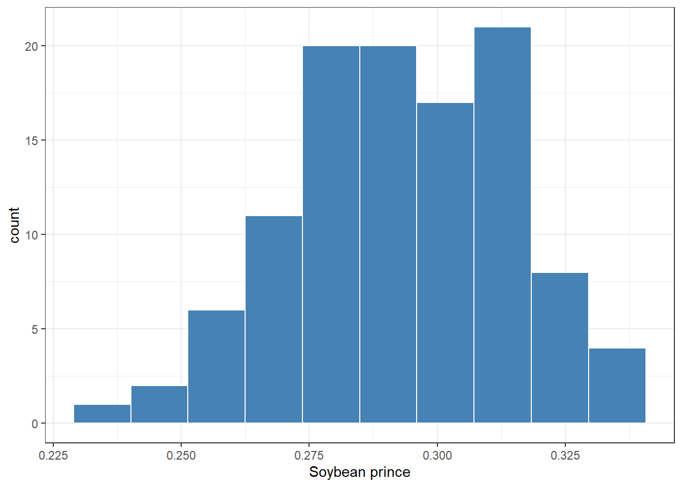

hist((sbr_price$price), prob = T)
curve(dnorm(x, mean(sbr_price$price), sd(sbr_price$price)),0.15,0.35, add = T)

plot(ecdf(sbr_price$price))
curve(pnorm(x, mean(sbr_price$price), sd(sbr_price$price)),0.2,0.35, add = T)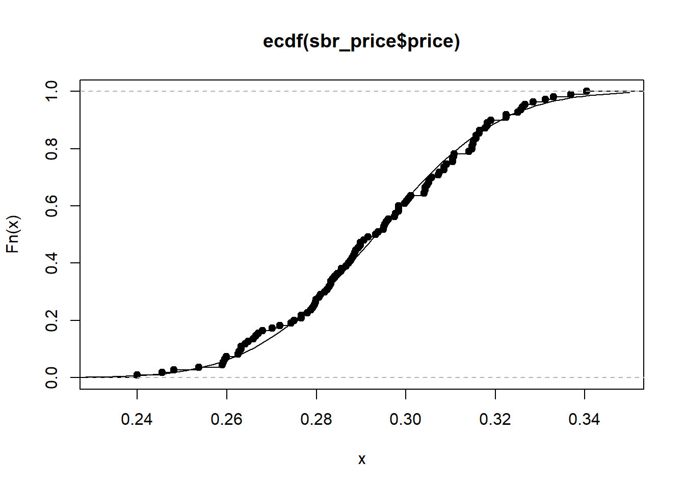

Mean and median

mean(sbr_price$price)

## [1] 0.2932792

median(sbr_price$price)

## [1] 0.2935692

Shapiro

shapiro.test(sbr_price$price)

## 
##  Shapiro-Wilk normality test
## 
## data:  sbr_price$price
## W = 0.99021, p-value = 0.6164

Kolmogorov-Smirnov Test

Fx = environment(ecdf(sbr_price$price))$y
x= environment(ecdf(sbr_price$price))$x
ks.test(Fx, pnorm(x, mean(sbr_price$price), sd(sbr_price$price)))

## 
##  Two-sample Kolmogorov-Smirnov test
## 
## data:  Fx and pnorm(x, mean(sbr_price$price), sd(sbr_price$price))
## D = 0.054545, p-value = 0.9967
## alternative hypothesis: two-sided

plot(Fx, pnorm(x, mean(sbr_price$price), sd(sbr_price$price)))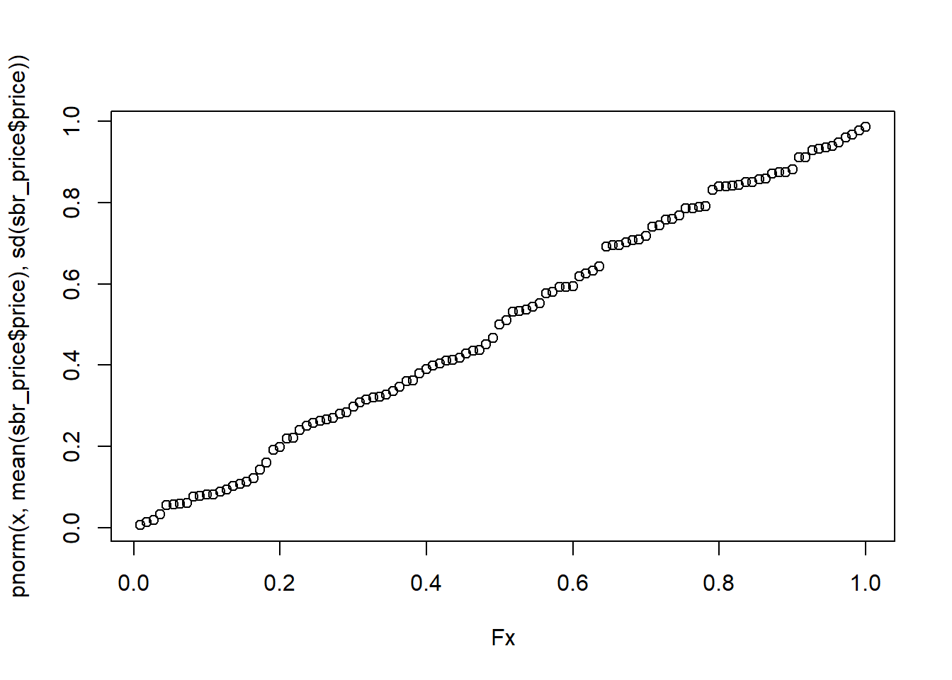

Vizualization

price_plot = sbr_price %>% 
  ggplot(aes(price))+
 geom_histogram(aes(y = ..density..),bins = 10, color = "white", fill = "#1C8C20")+
   stat_function(fun=function(x) dnorm(x, mean(sbr_price$price), sd(sbr_price$price)), color= "black", size = 1.2)+
  theme_bw()+
  labs(x="Soybean price (US$/kg)", y = "Density")+
  scale_x_continuous(breaks = seq(0,1,by=0.025))
price_plot

# ggsave("figs/sev_dist.png", dpi=600, height = 3, width = 4)

Regression coeficients

import data

Importing regression Slope and intercept data from the relationship between SBR severity and yield

damage_data = read_excel("data/dados histograma.xlsx") %>% 
  mutate(Slope = b1,
         Intercept = b0) %>% 
  dplyr::select(-b1,-b0)
head(damage_data)

Empirical distribution

Visualizando os hitogramas do slope e intercepto

damage_data %>% 
  gather(2:3, key = "par", value = "value") %>% 
  ggplot(aes(value))+
  geom_histogram(bins = 10, color = "gray40", fill = "gray90")+
  facet_wrap(~par, scales = "free_x")+
  theme_bw()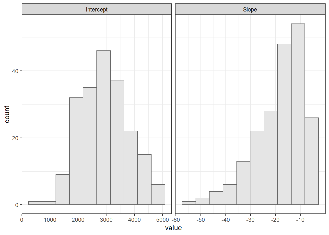

Regression lines

  ggplot() +
  geom_point(aes(x = 0:100, y = seq(0,5000,by = 50)), color = NA)+
  geom_abline(data =damage_data, aes(slope = Slope, intercept = Intercept),
              alpha = 0.5, color = "gray")+
  geom_abline(intercept = 2977,slope = -18, size = 1.2)+
  geom_abline(intercept = 2862,slope = -19.4 , size = .51, linetype = 2)+
  geom_abline(intercept = 3093,slope = -16.6, size = .51, linetype = 2)+
  
  labs(x = "SBR Severity (%)", y = "Yield (kg/ha) ")+
  theme_base()

## Warning: Removed 101 rows containing missing values (geom_point).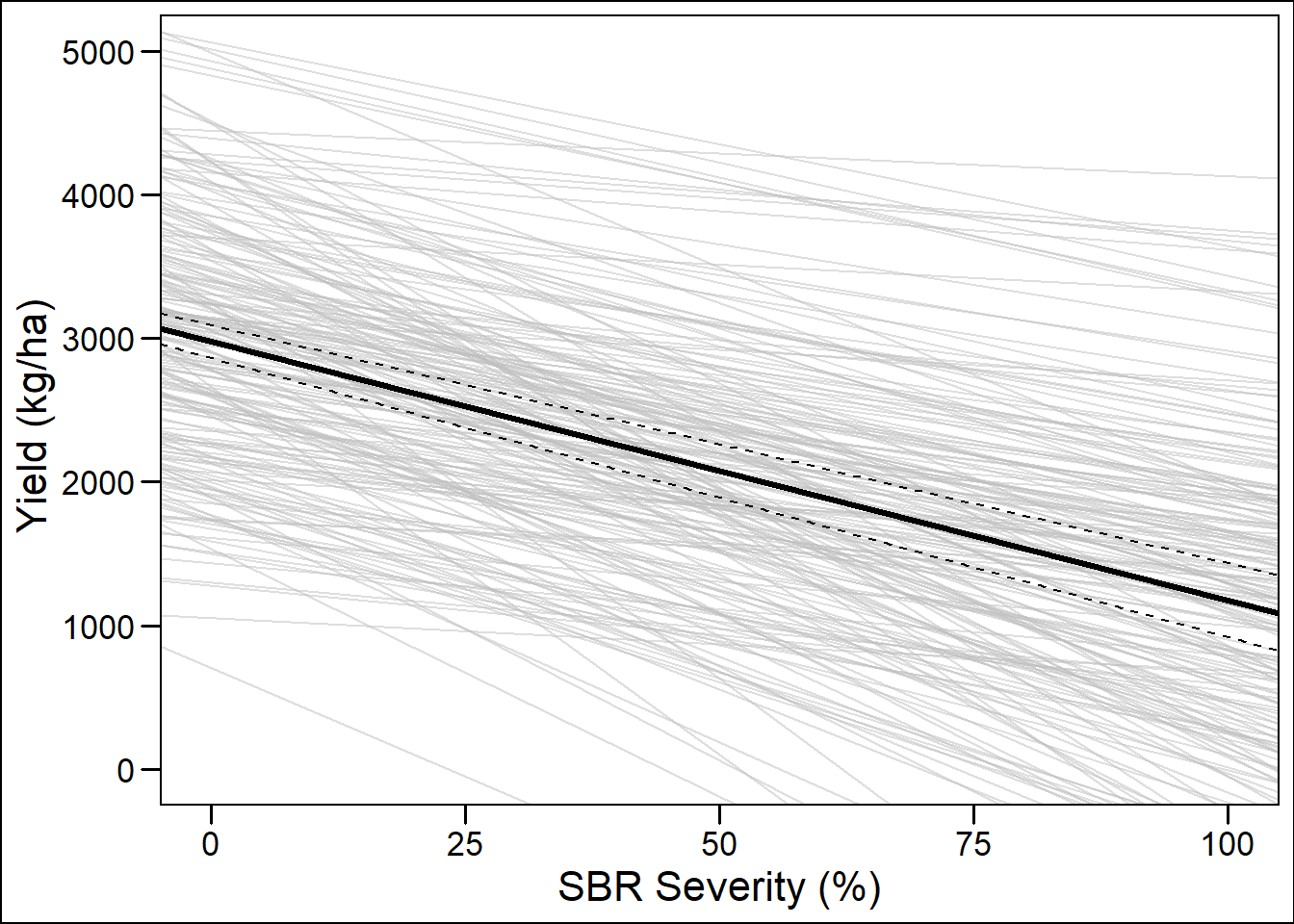

correlation

Correlation between slope and intercept

correlation(damage_data$Slope, damage_data$Intercept)

## 
## Pearson's product-moment correlation
## 
## data: damage_data$Slope and damage_data$Intercept 
## t = -3.144296 , df = 202 , p-value = 0.001915808 
## alternative hypothesis: true rho is not equal to 0
## sample estimates:
## cor
##  -0.2160089

plot

corr_emp_plot = damage_data %>% 
  ggplot(aes(Intercept, Slope))+
  geom_point(color = "black", size =2, alpha =0.5)+
  # geom_density2d_filled()+
  geom_smooth(method = "lm", se = F, color ="Red", size=1.2, fullrange=TRUE)+
  theme_light()+
  labs(title = "Empirical: r = -0.216")+
  coord_cartesian(
    xlim = c(0,6000),
    ylim = c(-75,0)
  )
corr_emp_plot

## `geom_smooth()` using formula 'y ~ x'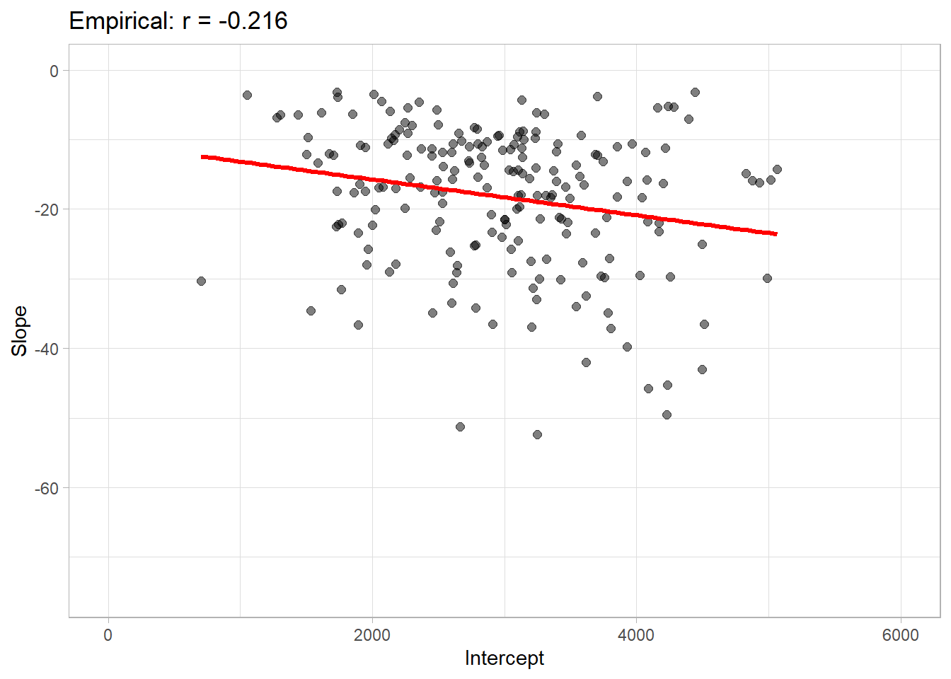

Cumulative density

Intercept

mean_intercept = mean(damage_data$Intercept)
sd_intercept = sd(damage_data$Intercept)

plot(ecdf(damage_data$Intercept))
curve(pnorm(x, mean_intercept,sd_intercept), 1000,5000, add = T, col = "red")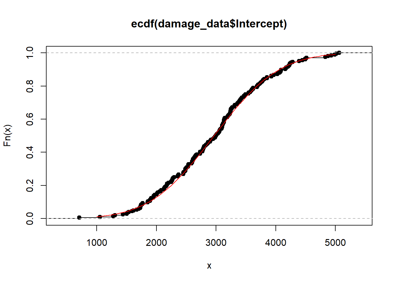

Kolmogorov-Smirnov Test

Fx = environment(ecdf(damage_data$Intercept))$y
x= environment(ecdf(damage_data$Intercept))$x
ks.test(Fx, pnorm(x, mean(damage_data$Intercept), sd(damage_data$Intercept)))

## 
##  Two-sample Kolmogorov-Smirnov test
## 
## data:  Fx and pnorm(x, mean(damage_data$Intercept), sd(damage_data$Intercept))
## D = 0.034314, p-value = 0.9997
## alternative hypothesis: two-sided

plot(Fx, pnorm(x, mean(damage_data$Intercept), sd(damage_data$Intercept)))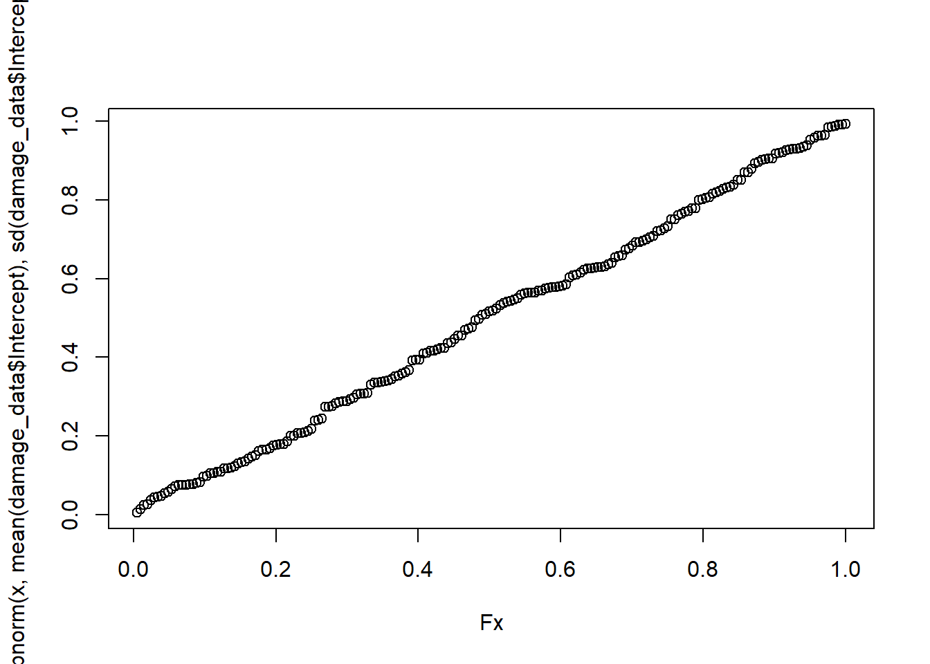

intercep_plot = damage_data %>% 
  ggplot(aes(Intercept))+
  geom_histogram(aes(y = ..density..),bins = 10, color = "white", fill = "#FF4917")+
  stat_function(fun=function(x) dnorm(x, mean_intercept, sd_intercept), color ="black", size =1.2)+
  theme_bw()+
  labs(x="Intercept (kg/ha)", y = "Density")
intercep_plot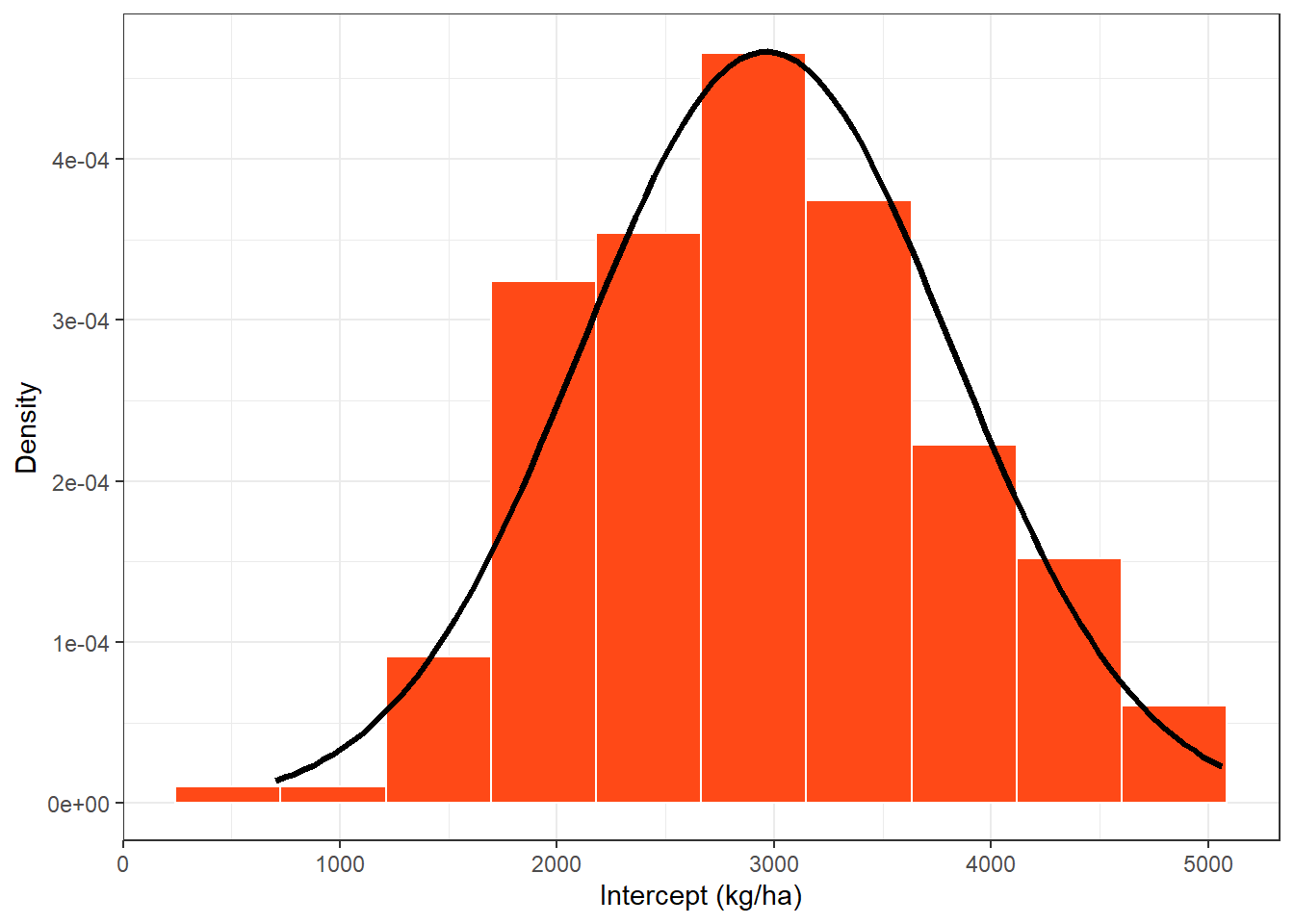

Slope

mean_slope = mean(damage_data$Slope)
sd_slope = sd(damage_data$Slope)

plot(ecdf(damage_data$Slope))
curve(pnorm(x, mean_slope, sd_slope), -60,5, add = T, col = "red")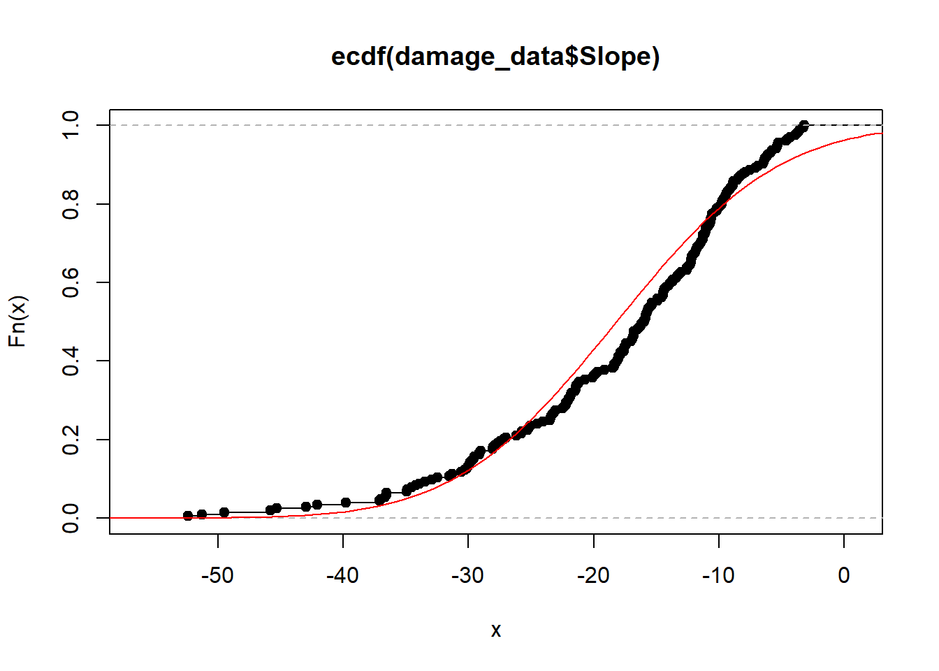

Modeling

Fitting gamma distribution to the empirical cumulative density of the slope data

Fx =environment(ecdf(-damage_data$Slope))$y
x = environment(ecdf(-damage_data$Slope))$x

slope_reg = nlsLM(Fx ~ pgamma(x, shape, rate,log = FALSE) ,
      start = c(shape = 2.5, rate = 0.13),
      control = nls.lm.control(maxiter = 1024))
summary(slope_reg)

## 
## Formula: Fx ~ pgamma(x, shape, rate, log = FALSE)
## 
## Parameters:
##       Estimate Std. Error t value Pr(>|t|)    
## shape 3.044261   0.031275   97.34   <2e-16 ***
## rate  0.168269   0.001929   87.22   <2e-16 ***
## ---
## Signif. codes:  0 '***' 0.001 '**' 0.01 '*' 0.05 '.' 0.1 ' ' 1
## 
## Residual standard error: 0.014 on 201 degrees of freedom
## 
## Number of iterations to convergence: 4 
## Achieved convergence tolerance: 1.49e-08

Kolmogorov-Smirnov Test

shape = summary(slope_reg)$coef[1]
rate = summary(slope_reg)$coef[2]

Fx =environment(ecdf(-damage_data$Slope))$y
x = environment(ecdf(-damage_data$Slope))$x
ks.test(Fx, pgamma(x, shape, rate))

## 
##  Two-sample Kolmogorov-Smirnov test
## 
## data:  Fx and pgamma(x, shape, rate)
## D = 0.034483, p-value = 0.9997
## alternative hypothesis: two-sided

shape = summary(slope_reg)$coef[1]
rate = summary(slope_reg)$coef[2]

slope_plot = damage_data %>% 
  ggplot(aes(Slope))+
 geom_histogram(aes(y = ..density..),bins = 10, color = "white", fill = "#159EE6")+
   stat_function(fun=function(x) dgamma(-x, shape, rate), size = 1.2, color = "black")+
  theme_bw()+
  labs(x="Slope (kg/p.p.)", y = "Density")
slope_plot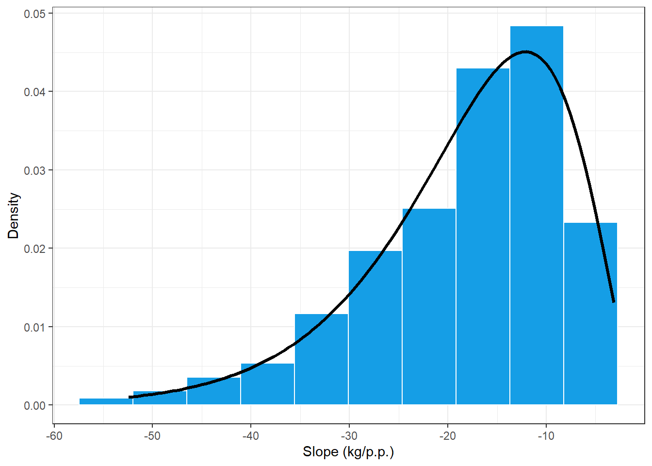

Kolmogorov-Smirnov Test

ks.test(Fx,pgamma(x, shape, rate))

## 
##  Two-sample Kolmogorov-Smirnov test
## 
## data:  Fx and pgamma(x, shape, rate)
## D = 0.034483, p-value = 0.9997
## alternative hypothesis: two-sided

Multivariate Simulation using copula

Simulating two normal distributions correlated #### Function

######################################
gera.norm.bid.geral<-function(tamanho.amostra,correlacao,m1,m2,sigma1,sigma2)
{
  ro<-correlacao
  n<-tamanho.amostra
  x<-matrix(0,n,2)
  for (i in 1:n)
  {x[i,1]<-rnorm(1,m1,sigma1)
  x[i,2]<-rnorm(1,m2+ro*sigma1/sigma2*(x[i,1]-m1),sigma2*(sqrt(1-ro^2)))
  }
  return(x)
}

Test for correlation of 0.9

#testando
j<-gera.norm.bid.geral(1000,0.9,0,0,1,1)

plot(j[,1],j[,2])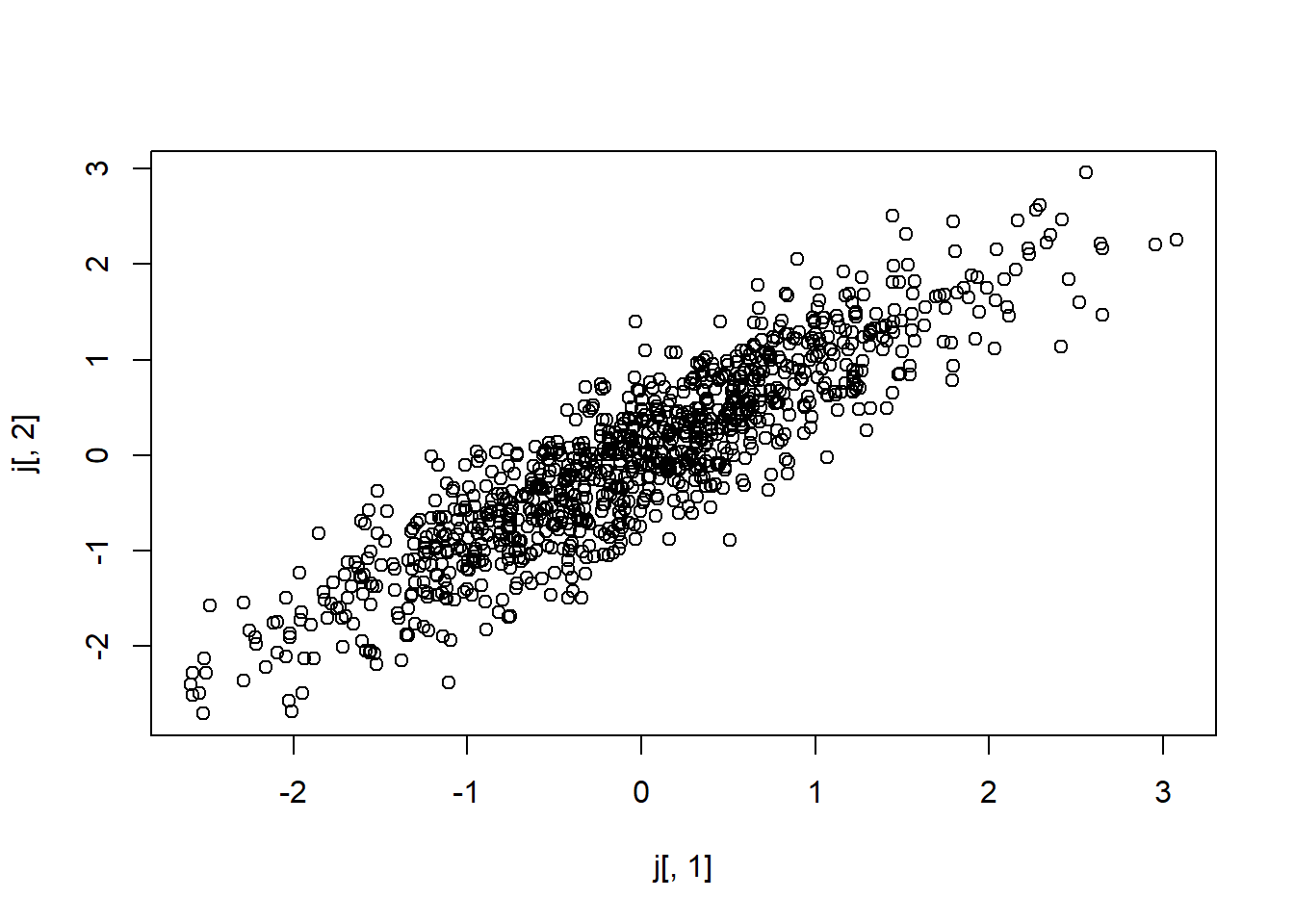

For our data, we will use the positive correlation, becouse we want positive values of slope

#testando
j<-gera.norm.bid.geral(10000,0.2160089,0,0,1,1)

plot(j[,1],j[,2])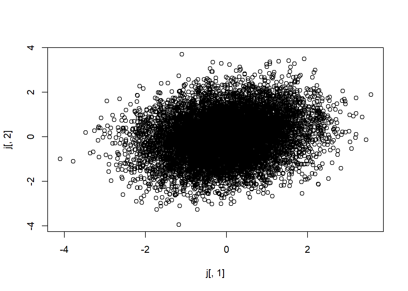

Intercept

Now we obtaing the probabilities from first distribution and insert in the quantiles function for the normal distribution of the intercept

b0 = pnorm(j[,2])
b0_t = qnorm(b0, 2977, 58.9*sqrt(210))
hist(b0_t, prob = T)
curve(dnorm(x, mean_intercept, sd_intercept), 0, 6000, add = T)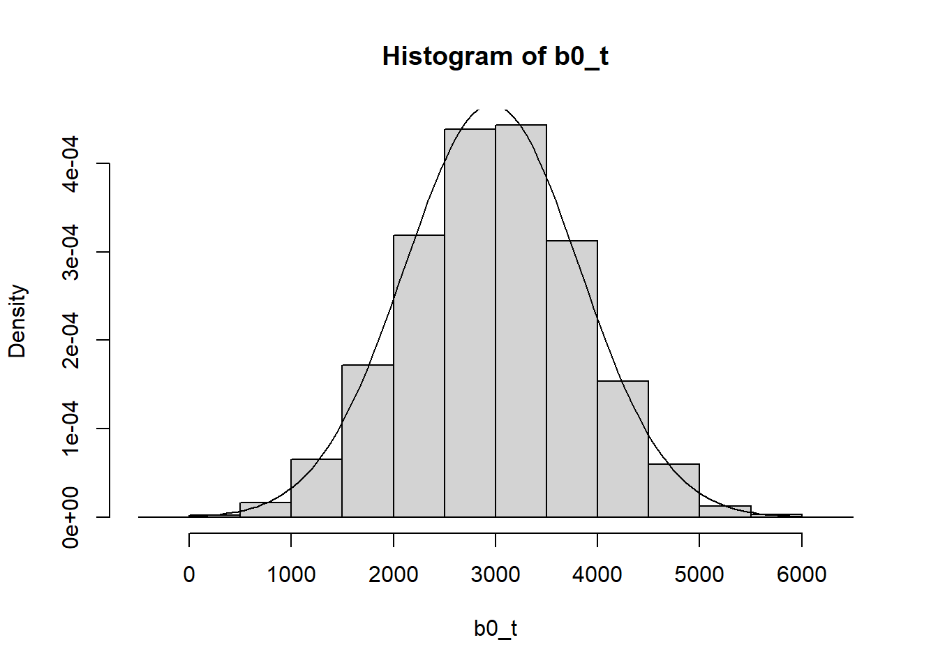

Slope

Now we obtaing the probabilities from first distribution and insert in the quantiles function for the gamma ditribution and multiply for -1 for obtain the negative outputs of the coeficient

b1 = pnorm(j[,1])
b1_t = qgamma(b1, shape, rate = rate)*-1
hist(b1_t, prob = T)
curve(dgamma(-x,shape=shape, rate = rate), -60,0, add = T)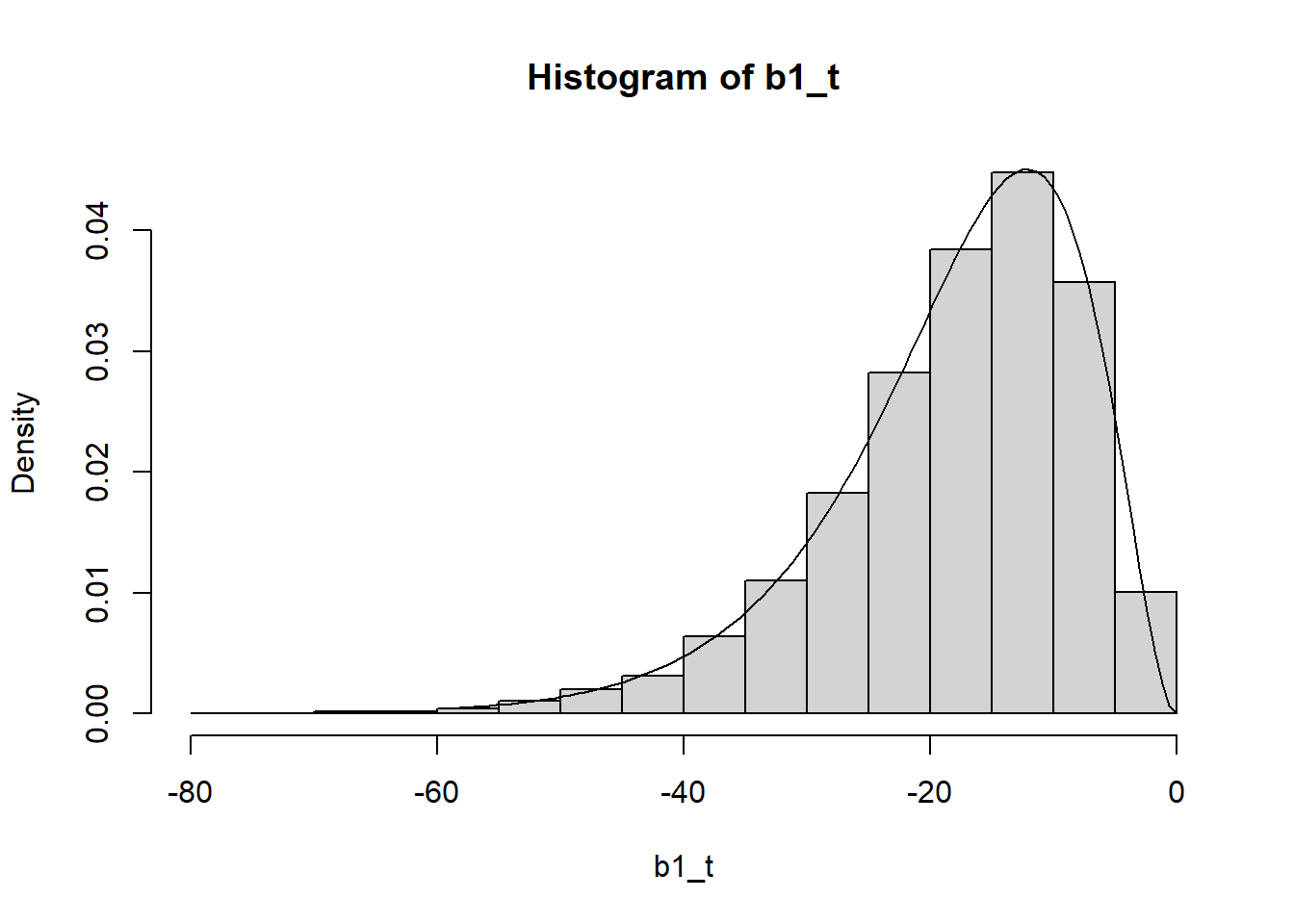

Now we recalculate the correlation between the simulated coeficients. It matchs!

correlation(b1_t, b0_t)

## 
## Pearson's product-moment correlation
## 
## data: b1_t and b0_t 
## t = -21.87086 , df = 9998 , p-value = 0 
## alternative hypothesis: true rho is not equal to 0
## sample estimates:
## cor
##  -0.2136786

Viz. the correlation

corr_sim_plot = data.frame(b0_t,b1_t ) %>%
  mutate(alfa =(b1_t/b0_t)*100 ) %>% 
  filter(alfa > -3 & alfa < 0) %>% 
ggplot(aes(b0_t,b1_t ))+
  geom_point( size =2, color = "orange", alpha =0.3)+
  # geom_density_2d(color = "black")+
  geom_smooth(method = lm, color = "red", se = F, size = 1.2)+
  theme_light()+
  labs(y= "Slope",
       x = "Intercept",
       title = "Simulated: r = -0.204")+
  coord_cartesian(
    xlim = c(0,6000),
    ylim = c(-75,0)
  )
corr_sim_plot

## `geom_smooth()` using formula 'y ~ x'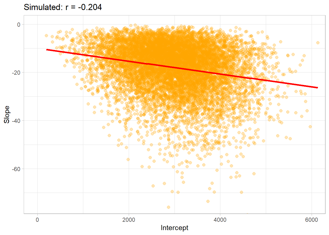

Combo distributions

# plot_grid(sev_dist_plot,price_plot, intercep_plot, slope_plot, labels = "AUTO", nrow =2)

(sev_dist_plot+price_plot)/
  (intercep_plot+slope_plot)+
  # (corr_emp_plot+corr_sim_plot)+
  plot_annotation(tag_levels = 'A')&
  theme(plot.title = element_text(size =8))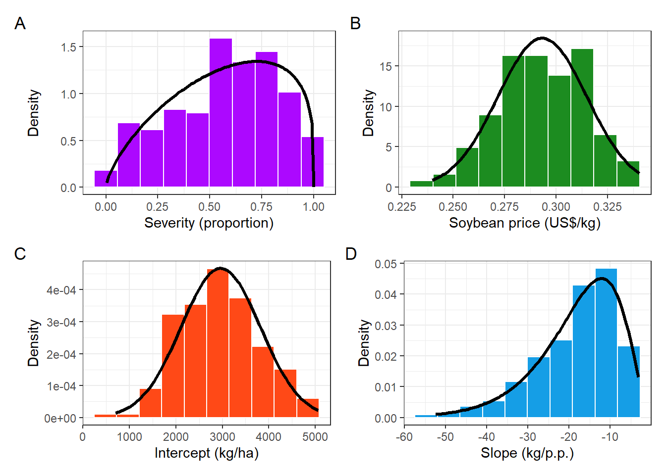

ggsave("figs/coef_dist.png", dpi = 600, height = 5, width = 6)
ggsave("figs/coef_dist.pdf", dpi = 600, height = 5, width = 6)

Relative yield loss

Here we calculate the yield relative loss due to SBR severity using the original data set

empiric_ryl= damage_data %>% 
  mutate(cc = (Slope/Intercept)*100) %>% 
  filter( cc > -3 & cc <0 )
head(empiric_ryl)

stat_emp_ryl =empiric_ryl%>% 
  summarise(data = "empirical",
            mean =  mean(cc),
            median =  median(cc),
            variance = var(cc))

real_RYL= empiric_ryl %>% 
  ggplot(aes(cc))+
 geom_histogram(aes(y = ..density..),bins = 10, color = "white", fill = "black")+
  scale_y_continuous(limits = c(0,1.4),breaks =  seq(0, 1.4,by = 0.4))+
  geom_vline(data = stat_emp_ryl, aes(xintercept = mean, color = "Mean"),size =1)+
  geom_vline(data = stat_emp_ryl, aes(xintercept = median, color = "Median"),size =1)+
  theme_bw()+
  scale_color_calc()+
  labs(x = "Relative yield loss (%/p.p.)",
       y = "Density",
       color = "",
       title = "Empirical")+
  xlim(-3,0.2)+
  theme(legend.position = "top")
real_RYL

## Warning: Removed 2 rows containing missing values (geom_bar).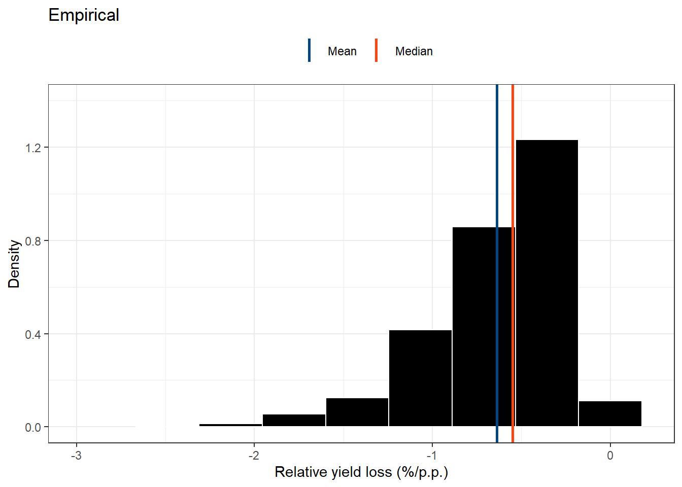

And here we calculate the relative yield loss due to SBR severity using the simulated data set

simul_ryl = data.frame(b0_t, b1_t, cc = (b1_t/b0_t)*100) %>% 
  filter( cc > -3 & cc <0 )
head(simul_ryl)

stat_suml_ryl = simul_ryl%>% 
  summarise(data = "Simulated",
            mean =  mean(cc),
            median =  median(cc),
            variance = var(cc))

simul_RYL =simul_ryl %>% 
  ggplot(aes(cc))+
 geom_histogram(aes(y = ..density..),bins = 10, color = "white", fill = "orange")+
  scale_y_continuous(limits = c(0,1.4),breaks =  seq(0, 1.4,by = 0.4))+
  geom_vline(data = stat_suml_ryl, aes(xintercept = mean, color = "Mean"),size =1)+
  geom_vline(data = stat_suml_ryl, aes(xintercept = median, color = "Median"),size =1)+
  theme_bw()+
  scale_color_calc()+
  labs(x = "Relative yield loss (%/p.p.)",
       y = "Density",
       color ="",
       title = "Simulated")+
  xlim(-3,0.2)+
  theme(legend.position = "top")
simul_RYL

## Warning: Removed 2 rows containing missing values (geom_bar).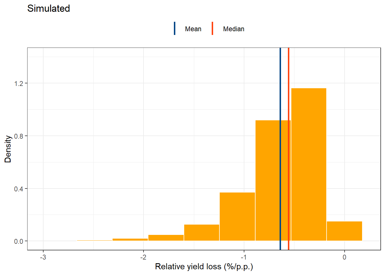

Comparision of mean, median and variance

damage_data %>% 
  mutate(cc = (Slope/Intercept)*100) %>% 
  filter( cc > -3 & cc <0 ) %>% 
  summarise(data = "empirical",
            mean =  mean(cc),
            median =  median(cc),
            variance = var(cc)) %>% 
  bind_rows(
    data.frame(b0_t, b1_t, cc = (b1_t/b0_t)*100) %>% 
  filter( cc > -3 & cc <0 ) %>% 
  summarise(data = "Simulated",
            mean =  mean(cc),
            median =  median(cc),
            variance = var(cc))
  )

Kolmogorov-Smirnov Test

actual_cc = damage_data %>% 
  mutate(cc = (Slope/Intercept)*100)

simulated_cc = data.frame(b0_t, b1_t, cc = (b1_t/b0_t)*100) %>% 
  filter( cc > -3 & cc <0 )

Distribution

ks.test(actual_cc$cc, simulated_cc$cc)

## 
##  Two-sample Kolmogorov-Smirnov test
## 
## data:  actual_cc$cc and simulated_cc$cc
## D = 0.050452, p-value = 0.6889
## alternative hypothesis: two-sided

cummulative distribution

fx_actual = environment(ecdf(actual_cc$cc))$y
fx_simu = environment(ecdf(simulated_cc$cc))$y
ks.test((fx_actual),(fx_simu))

## Warning in ks.test((fx_actual), (fx_simu)): p-value will be approximate in the
## presence of ties

## 
##  Two-sample Kolmogorov-Smirnov test
## 
## data:  (fx_actual) and (fx_simu)
## D = 0.004899, p-value = 1
## alternative hypothesis: two-sided

ecdf_damage = ggplot()+
  stat_ecdf(aes(simulated_cc$cc,color = "Simulated"), size=1.2,geom = "step")+
  stat_ecdf(aes(actual_cc$cc, color = "Empirical"), size=1.2,geom = "step")+
  theme_bw()+
  scale_color_manual(values = c("black","orange"))+
  labs(y = "Probability",
       x = "Relative percent yield loss",
       color ="",
       title = "Cumulative distribution function")+
  theme(legend.position = "top",
        legend.background = element_blank())
ecdf_damage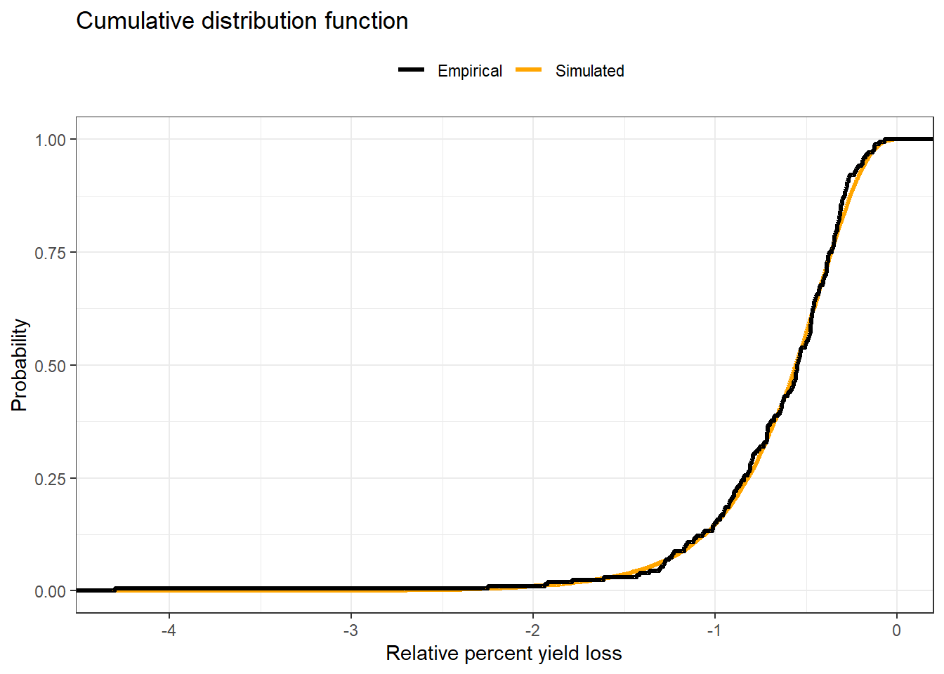

Combo Yield loss

((corr_emp_plot/corr_sim_plot)|(real_RYL/simul_RYL)+plot_layout(guides = 'collect')| ecdf_damage ) +
  # plot_layout(heights = c(1,1,0.5))+
  plot_annotation(tag_levels = 'A') & 
  
  theme(legend.position = 'bottom',
        plot.title = element_text(size=9),
        legend.key.size= unit(3, "mm"),
        legend.text =  element_text(size = 7))

## `geom_smooth()` using formula 'y ~ x'
## `geom_smooth()` using formula 'y ~ x'

## Warning: Removed 2 rows containing missing values (geom_bar).

## Warning: Removed 2 rows containing missing values (geom_bar).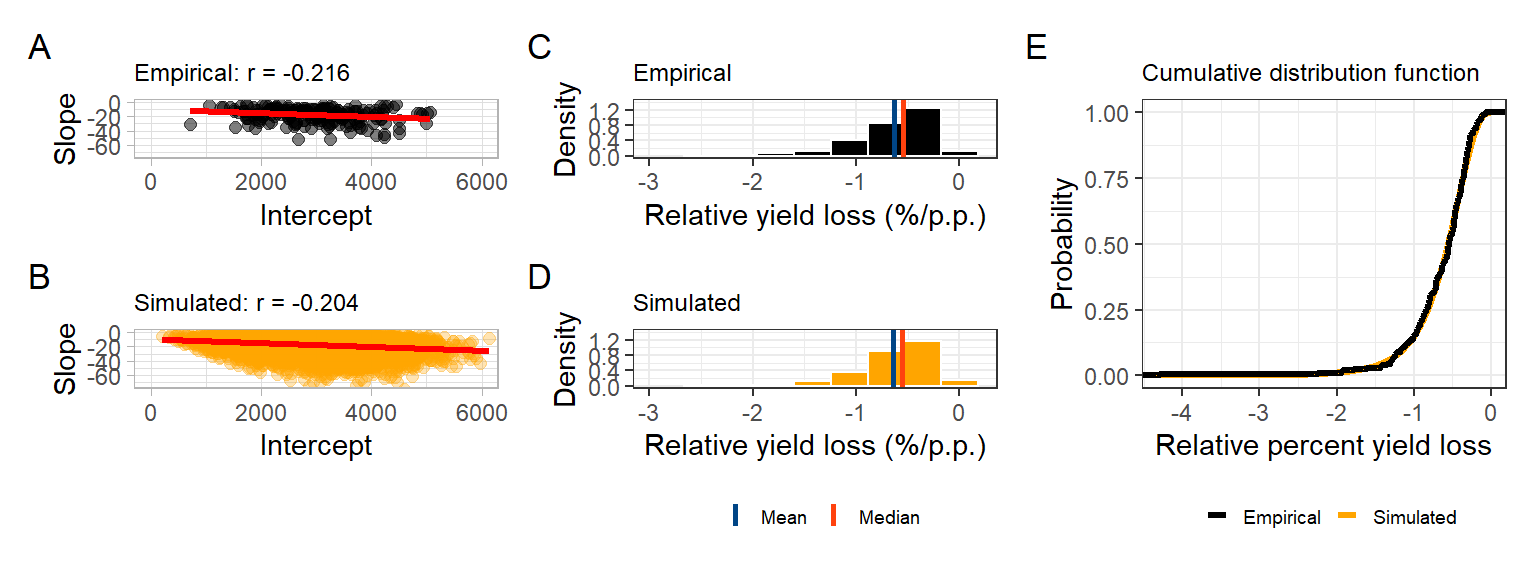

ggsave("figs/RYL.png", dpi = 600, height = 5, width = 10)

## `geom_smooth()` using formula 'y ~ x'
## `geom_smooth()` using formula 'y ~ x'

## Warning: Removed 2 rows containing missing values (geom_bar).

## Warning: Removed 2 rows containing missing values (geom_bar).

ggsave("figs/RYL.pdf", dpi = 600, height = 5, width = 10)

## `geom_smooth()` using formula 'y ~ x'
## `geom_smooth()` using formula 'y ~ x'

## Warning: Removed 2 rows containing missing values (geom_bar).

## Warning: Removed 2 rows containing missing values (geom_bar).

Simulations

set.seed(1)
n=40000
lambda = seq(0,1, by=0.05)
fun_price = seq(-10, 260, by=15)
n_aplication = 1
operational_cost = 10  

comb_matrix = as.matrix(data.table::CJ(lambda,fun_price))
colnames(comb_matrix) = c("lambda","fun_price")
comb_matrix = cbind(comb_matrix,operational_cost, n_aplication)
C = comb_matrix[,"n_aplication"]*(comb_matrix[,"operational_cost"]+comb_matrix[,"fun_price"] )
comb_matrix = cbind(comb_matrix,C)

N = length(comb_matrix[,1])*n
big_one = matrix(0, ncol = 12, nrow =N)
big_one[,1] = rep(comb_matrix[,1],n)
big_one[,2] = rep(comb_matrix[,2],n)
big_one[,3] = rep(comb_matrix[,3],n)
big_one[,4] = rep(comb_matrix[,4],n)
big_one[,5] = rep(comb_matrix[,5],n)

set.seed(1)
sn = rbeta(N, 1.707, 1.266)
sf = sn*(1-big_one[,1])
# simulating the coeficientes 
set.seed(1)
normal_correlated<-gera.norm.bid.geral(N,0.21,0,0,1,1)
b0_n = pnorm(normal_correlated[,2])
b1_n = pnorm(normal_correlated[,1])
b0 = qnorm(b0_n, mean_intercept,sd_intercept)
b1 = -qgamma(b1_n, shape, rate,)
rm(b0_n,b1_n,normal_correlated)
# b0[b0<0] = 0.0001
# Calculating the alha coeficient
alfa = (b1/b0)*100
# alfa[alfa > 0] = 0
# alfa[alfa < -3] = -3

# Calculating yield gain
# yn = b0*(1+sn*alfa) # Yield  non-treated
# yf = b0*(1+sf*alfa) # Yield  treated
yn  = b0 - (-alfa*b0*sn)
yf  = b0 - (-alfa*b0*sf)
# yn[yn<0] = 0
# yf[yf<0] = 0
# yield_gain = yf-yn # yield gain
# yield_gain_perc = (1-(yn/yf))*100


# Simulating soybean price
set.seed(1)
soy_price = rnorm(N, mean(sbr_price$price),sd(sbr_price$price))
# income = yield_gain*soy_price # calculating the income

big_one[,6] = yn
big_one[,7] = yf
big_one[,8] = soy_price
big_one[,9] = b1
big_one[,10] = alfa
big_one[,11] = b0
big_one[,12] = sn
colnames(big_one)  = c("lambda","fun_price","operational_cost","n_aplication","C","yn","yf","soy_price","b1","alfa","b0", "sn")

big_one_df = as.data.frame(big_one) %>% 
  filter(b0>=0) %>% 
  filter(yn>0) %>% 
  filter(alfa > -3 & alfa < 0) %>% 
  mutate(yield_gain = yf-yn,
         # yield_gain_perc = ((yf - yn)/yn)*100,
         yield_gain_perc = ((yf/yn)-1)*100,
         income = yield_gain*soy_price,
         CP = C/soy_price,
         # profit = (yield_gain>=CP)*1,
         profit = (income>=C)*1)

Breacking even

Tetris

big_one_df %>% 
  # mutate(sev_class = case_when(sn > median(sn) ~ "High severity",
                                 # sn <= median(sn) ~ "Low severity")) %>% 
  filter(lambda >=0.3) %>%
  group_by(lambda, C) %>% 
  summarise(n=n(),sumn = sum(profit), prob = sumn/n) %>%
  # filter(prob>0.5) %>%
  mutate(prob2 = case_when(prob < 0.50 ~ "Pr(I \u2265 C) \u2264 0.5 ",
                          prob >= 0.50 ~ "Pr(I \u2265 C) > 0.5")) %>% #,
  # #                         prob >= 0.75 ~ "75% \u2264 p < 100% "  )) %>% 
  ggplot(aes(as.factor(lambda*100),as.factor(C), fill = prob, 
             # color = prob2
             ))+
  geom_tile(size = 0.5, color ="white")+
  scale_fill_viridis_b(option ="B", direction = -1)+
  # scale_fill_manual(values = c("darkred",  "steelblue"))+
  # scale_fill_gradient2(low = "#E60E00",mid = "#00030F", high = "#55E344",midpoint = 0.5)+
  scale_color_manual(values = c("#E60E00","#55E344"))+
  # scale_fill_gradient2(low = "red",mid = "black", high = "steelblue",midpoint = 0.5)+
  # scale_color_manual(values = c("red","steelblue")) + 
  guides(color = guide_legend(override.aes = list(size=2)))+
  # scale_fill_viridis_d(option = "B")+
  labs(x = "Fungicide efficacy (%)",
       y = "Fungicide + Application cost ($)",
       fill  = "Pr(I \u2265 C)",
       color ="" )+
  # facet_wrap(~sev_class)+
  theme_light()

## `summarise()` regrouping output by 'lambda' (override with `.groups` argument)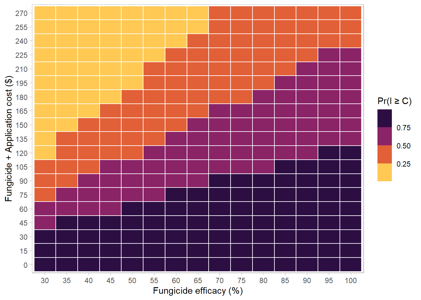

# ggsave("figs/tetris.png", dpi = 600, height = 5, width = 7)

Tetris 2

median(big_one_df$b0)

## [1] 2995.191

tetris_plot = function(s_class, y_class, pal =1){
big_one_df %>% 
  mutate(sev_class = case_when(sn > median(sn) ~ "High severity",
                                 sn <= median(sn) ~ "Low severity"),
      yield_class =  case_when(b0 > median(b0) ~ "High yield",
                                 b0 <= median(b0) ~ "Low yield")) %>%
    filter(lambda >=0.3) %>% 
  group_by(lambda, C, sev_class,yield_class) %>% 
  summarise(n=n(),sumn = sum(profit), prob = sumn/n) %>%
  mutate(prob = case_when(prob >= .75 ~ "\u2265 0.75",
                          prob < .75 & prob >= 0.5 ~ "0.50-0.75",
                          prob < .50 & prob >= .25 ~ "0.25-0.50",
                          prob < .25 ~ "< 0.25"),
         prob =factor(prob,level = c("< 0.25","0.25-0.50","0.50-0.75", "\u2265 0.75"))) %>%
    filter(sev_class== s_class,
           yield_class == y_class) %>% 
  ggplot(aes(as.factor(lambda*100),as.factor(C), fill = prob))+
  geom_tile(size = 0.25, color ="gray70")+
  scale_fill_brewer(palette = pal)+
  labs(x = "Fungicide efficacy (%)",
       y = "Fungicide + Application cost ($)",
       fill  = "Probability",
       color ="" )+
  # facet_grid(~sev_class)+
  guides(color = guide_legend(override.aes = list(size=2)))+
  theme_light()+
  theme(text = element_text(size = 10),
        legend.position = "bottom",
        axis.text = element_text(size = 7),
        panel.spacing = unit(1.75, "lines"),
        strip.background =element_rect(fill="NA"),
        strip.text = element_text(color = "black", size =12))
}

tetris_Sh_Sh = tetris_plot(s_class = "High severity",
                          y_class = "High yield",pal =1)+
  labs(title = "High severity",
       subtitle = "High yield")

## `summarise()` regrouping output by 'lambda', 'C', 'sev_class' (override with `.groups` argument)

tetris_Sl_Yh = tetris_plot(s_class = "Low severity",
                          y_class = "High yield",pal =1
                         )+
  labs(title = "Low severity",
       subtitle = "High yield")

## `summarise()` regrouping output by 'lambda', 'C', 'sev_class' (override with `.groups` argument)

tetris_Sh_Yl = tetris_plot(s_class = "High severity",
                          y_class = "Low yield",pal =2
                         )+
  labs(title = "High severity",
       subtitle = "Low yield")

## `summarise()` regrouping output by 'lambda', 'C', 'sev_class' (override with `.groups` argument)

tetris_Sl_Sh = tetris_plot(s_class = "Low severity",
                          y_class = "Low yield",pal =2
                         )+
  labs(title = "Low severity",
       subtitle = "Low yield")

## `summarise()` regrouping output by 'lambda', 'C', 'sev_class' (override with `.groups` argument)

Combo tetris

((tetris_Sh_Sh+tetris_Sl_Yh)+plot_layout(guides = "collect"))/((tetris_Sh_Yl+tetris_Sl_Sh)+
   plot_layout(guides = "collect"))+
  plot_annotation(tag_levels = 'A')&
  theme(legend.position = "bottom",
        plot.title = element_text(size = 8),
        plot.subtitle = element_text(size = 8))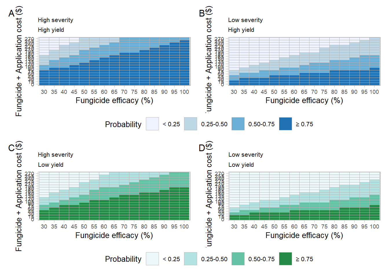

ggsave("figs/box_classes.png", dpi = 500, height = 8.5, width = 7.5)
ggsave("figs/box_classes.pdf", dpi = 500, height = 8.5, width = 7.5)

Yield gain

Absolute gain

overal_yg = big_one_df %>%
  mutate(sev_class = " Overall") %>% 
  group_by(lambda,sev_class) %>% 
  summarise(yield_gain_median = median(yield_gain),
            yield_gain_mean = mean(yield_gain),
            up_95 = quantile(yield_gain, 0.975),
            low_95 = quantile(yield_gain, 0.025),
            up_75 = quantile(yield_gain, 0.75),
            low_75 = quantile(yield_gain, 0.25))

## `summarise()` regrouping output by 'lambda' (override with `.groups` argument)

# m_absol = lm(yield_gain ~ lambda, big_one_df %>% mutate(lambda=lambda*100))
# summary(m_absol)

over_gg_kg = overal_yg %>% 
  ggplot(aes(lambda*100,yield_gain_mean))+
  geom_line(aes(lambda*100, low_95),
              linetype = 2,
            size = 0.7,
            fill = NA)+
  geom_line(aes(lambda*100, up_95),
              linetype = 2,
            size = 0.7,
            fill = NA)+
  geom_line(size = 1.2, aes(lambda*100,yield_gain_median))+
  # scale_linetype_manual(values=c(1,2))+
  theme_light()+
  # geom_abline(slope = 9.61, intercept = -0.1 )+
  # coord_equal()+
  labs(x = "Fungicide efficacy (%)",
       y = "Yield gain (kg/ha)",
       color = "Fungicide mixture", #(Dalla lana et al., 2018)
       linetype = "", fill = "")

## Warning: Ignoring unknown parameters: fill

## Warning: Ignoring unknown parameters: fill

over_gg_kg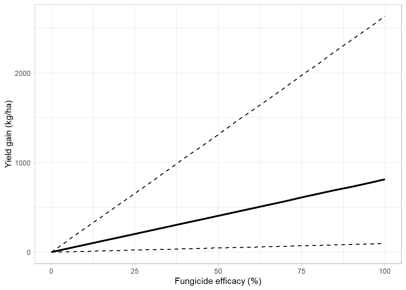

ygain_plot = function(s_class){
big_one_df %>% 
  mutate(sev_class = case_when(sn > median(sn) ~ "High severity",
                                 sn <= median(sn) ~ "Low severity"),
      yield_class =  case_when(b0 > median(b0) ~ "High yield",
                                 b0 <= median(b0) ~ "Low yield")) %>%
  group_by(lambda, sev_class,yield_class ) %>% 
  summarise(yield_gain_median = median(yield_gain),
            yield_gain_mean = mean(yield_gain),
            up_95 = quantile(yield_gain, 0.975),
            low_95 = quantile(yield_gain, 0.025),
            up_75 = quantile(yield_gain, 0.75),
            low_75 = quantile(yield_gain, 0.25)) %>% 
  mutate(sev_class = factor(sev_class, levels = c("Low severity","High severity"))) %>%
    filter(sev_class ==s_class ) %>% 
  ggplot(aes(lambda*100,yield_gain_mean))+
  geom_line(aes(lambda*100, low_95, color = yield_class),
              linetype = 2,
            size = 0.7,
            fill = NA)+
  geom_line(aes(lambda*100, up_95,color = yield_class),
              linetype = 2,
            size = 0.7,
            fill = NA)+
  geom_line(size = 1.2, aes(lambda*100,yield_gain_median,color = yield_class))+
  # scale_color_manual(values = c("#009628","#8A0004"))+
  scale_color_manual(values = c("steelblue","#009628"))+
  theme_light()+
    coord_cartesian(ylim=c(0,3000))+
  labs(x = "Fungicide efficacy (%)",
       y = "Yield gain (kg/ha)",
       color = "Attainable Yield", #(Dalla lana et al., 2018)
       linetype = "")
}
high_sev_yg = ygain_plot(s_class = "High severity")+
  labs(title = "High severity")

## `summarise()` regrouping output by 'lambda', 'sev_class' (override with `.groups` argument)

## Warning: Ignoring unknown parameters: fill

## Warning: Ignoring unknown parameters: fill

low_sev_yg = ygain_plot(s_class = "Low severity")+
  labs(title = "Low severity")

## `summarise()` regrouping output by 'lambda', 'sev_class' (override with `.groups` argument)

## Warning: Ignoring unknown parameters: fill

## Warning: Ignoring unknown parameters: fill

high_sev_yg+low_sev_yg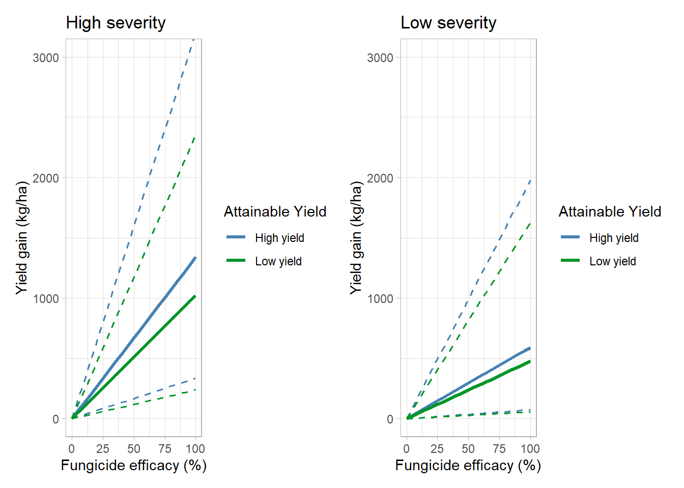

big_one_df %>%
  mutate(sev_class = case_when(sn > median(sn) ~ "High severity",
                                 sn <= median(sn) ~ "Low severity"),
      yield_class =  case_when(b0 > median(b0) ~ "High yield",
                                 b0 <= median(b0) ~ "Low yield")) %>%
  group_by(lambda, sev_class,yield_class ) %>% 
  summarise(yield_gain_mean = mean(yield_gain),
            yield_gain_median = median(yield_gain, na.rm = T),
            low_95 = quantile(yield_gain, 0.025),
            up_95 = quantile(yield_gain, 0.975),
            up_75 = quantile(yield_gain, 0.75),
            low_75 = quantile(yield_gain, 0.25)) %>% 
  bind_rows(overal_yg) %>% 
  filter(lambda==.75) %>% 
  arrange(yield_class)

## `summarise()` regrouping output by 'lambda', 'sev_class' (override with `.groups` argument)

Percent gain

overal_percet = big_one_df %>%
  mutate(sev_class = " Overall") %>% 
  group_by(lambda,sev_class) %>% 
  mutate(yield_gain_perc = case_when(yield_gain_perc>quantile(yield_gain_perc,0.999)~quantile(yield_gain_perc,0.999),
                                     yield_gain_perc<=quantile(yield_gain_perc,0.999) ~yield_gain_perc)) %>%
  summarise(yield_gain_mean = mean(yield_gain_perc,na.rm = T),
            yield_gain_median = median(yield_gain_perc,na.rm = T),
            low_95 = quantile(yield_gain_perc, 0.025,na.rm = T),
            up_95 = quantile(yield_gain_perc, 0.975,na.rm = T),
            up_75 = quantile(yield_gain_perc, 0.75,na.rm = T),
            low_75 = quantile(yield_gain_perc, 0.25,na.rm = T))  

## `summarise()` regrouping output by 'lambda' (override with `.groups` argument)

over_gg = overal_percet %>% 
  ggplot(aes(lambda*100,yield_gain_mean))+
  geom_line(aes(lambda*100, low_95),
              linetype = 2,
            size = 0.7,
            fill = NA)+
  geom_line(aes(lambda*100, up_95),
              linetype = 2,
            size = 0.7,
            fill = NA)+
  geom_line(size = 1.2, aes(lambda*100,yield_gain_median))+
  # scale_linetype_manual(values=c(1,2))+
  theme_light()+
  # coord_equal()+
  labs(x = "Fungicide efficacy (%)",
       y = "Yield gain %",
       color = "Fungicide mixture", #(Dalla lana et al., 2018)
       linetype = "", fill = "")+
  coord_cartesian(ylim = c(0,100), xlim = c(-10,100))

## Warning: Ignoring unknown parameters: fill

## Warning: Ignoring unknown parameters: fill

over_gg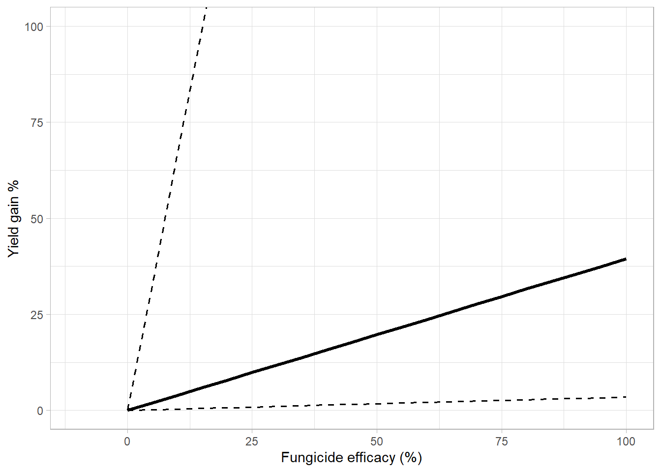

ygain_perc_plot = function(s_class){
big_one_df %>% 
  mutate(sev_class = case_when(sn > median(sn) ~ "High severity",
                                 sn <= median(sn) ~ "Low severity"),
      yield_class =  case_when(b0 > median(b0) ~ "High yield",
                                 b0 <= median(b0) ~ "Low yield")) %>%
  group_by(lambda, sev_class,yield_class ) %>% 
  summarise(yield_gain_median = median(yield_gain_perc),
            yield_gain_mean = mean(yield_gain_perc),
            up_95 = quantile(yield_gain_perc, 0.975),
            low_95 = quantile(yield_gain_perc, 0.025),
            up_75 = quantile(yield_gain_perc, 0.75),
            low_75 = quantile(yield_gain_perc, 0.25)) %>% 
  mutate(sev_class = factor(sev_class, levels = c("Low severity","High severity"))) %>%
    filter(sev_class ==s_class ) %>% 
  ggplot(aes(lambda*100,yield_gain_mean))+
  geom_line(aes(lambda*100, low_95, color = yield_class),
              linetype = 2,
            size = 0.7,
            fill = NA)+
  geom_line(aes(lambda*100, up_95,color = yield_class),
              linetype = 2,
            size = 0.7,
            fill = NA)+
  geom_line(size = 1.2, aes(lambda*100,yield_gain_median,color = yield_class))+
  # scale_color_manual(values = c("#009628","#8A0004"))+
  scale_color_manual(values = c("steelblue","#009628"))+

  theme_light()+
  labs(x = "Fungicide efficacy (%)",
       y = "Yield gain (%)",
       color = "Attainable Yield", 
       linetype = "", fill = "")+
  coord_cartesian(ylim = c(0,100))
}
high_sev_yg_perc = ygain_perc_plot(s_class = "High severity")+
  labs(title = "High severity")

## `summarise()` regrouping output by 'lambda', 'sev_class' (override with `.groups` argument)

## Warning: Ignoring unknown parameters: fill

## Warning: Ignoring unknown parameters: fill

low_sev_yg_perc = ygain_perc_plot(s_class = "Low severity")+
  labs(title = "Low severity")

## `summarise()` regrouping output by 'lambda', 'sev_class' (override with `.groups` argument)

## Warning: Ignoring unknown parameters: fill

## Warning: Ignoring unknown parameters: fill

Combo yied gain

(high_sev_yg+low_sev_yg)/
(high_sev_yg_perc+low_sev_yg_perc)+
  plot_layout(guides = "collect",
               heights = c(1,1))+
  plot_annotation(tag_levels = 'A')& 
  theme(plot.title = element_text(size =8))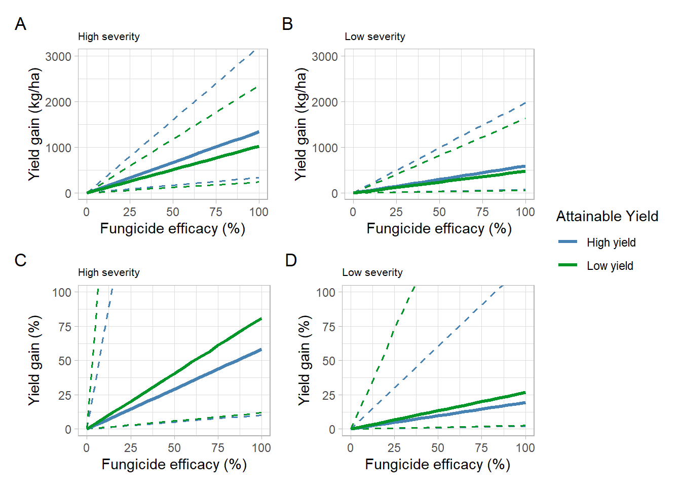

ggsave("figs/yield_gain_perc.png", dpi = 600, height = 6, width =8)
ggsave("figs/yield_gain_perc.pdf", dpi = 600, height = 6, width =8)

 big_one_df %>%
  mutate(sev_class = case_when(sn > median(sn) ~ "High severity",
                                 sn <= median(sn) ~ "Low severity"),
      yield_class =  case_when(b0 > median(b0) ~ "High yield",
                                 b0 <= median(b0) ~ "Low yield")) %>%
  group_by(lambda,sev_class,yield_class) %>%
  mutate(yield_gain_perc = case_when(yield_gain_perc>quantile(yield_gain_perc,0.999)~quantile(yield_gain_perc,0.999),
                                     yield_gain_perc<=quantile(yield_gain_perc,0.999) ~yield_gain_perc)) %>%
  summarise(yield_gain_mean = mean((yield_gain_perc),na.rm = T),
            yield_gain_median = median((yield_gain_perc),na.rm = T),
            low_95 = quantile((yield_gain_perc), 0.025,na.rm = T),
            up_95 = quantile((yield_gain_perc), 0.975,na.rm = T),
            up_75 = quantile((yield_gain_perc), 0.75,na.rm = T),
            low_75 = quantile((yield_gain_perc), 0.25,na.rm = T)) %>% 
  bind_rows(overal_percet)%>% 
  filter(lambda==0.75) %>% 
  arrange(yield_class)

## `summarise()` regrouping output by 'lambda', 'sev_class' (override with `.groups` argument)

Examples

Fungicide PICO+TEBU

n = 1000
# yield = rnorm(1000,682.11, 28.97)
efficacy = (1-exp(rnorm(1000,-1.204,0.0462)))

sev_n = rbeta(n, 1.707, 1.266)
sev_f = sev_n*(1-efficacy) 

normal_correlated<-gera.norm.bid.geral(n,0.21,0,0,1,1)
b0_n = pnorm(normal_correlated[,2])
b1_n = pnorm(normal_correlated[,1])
b0 = qnorm(b0_n, mean_intercept,sd_intercept)
b1 = -qgamma(b1_n, shape, rate,)
rm(b0_n,b1_n,normal_correlated)

# Calculating the alpha coeficient
alfa = (b1/b0)*100

# Calculating yield gain
yn  = b0 - (-alfa*b0*sev_n)
yf  = b0 - (-alfa*b0*sev_f)

cost = 125
soy_price = rnorm(n, mean(sbr_price$price),sd(sbr_price$price))

yield_gain = yf-yn
yield_gain_perc = ((yf - yn)/yn)*100
yield_gain_perc = ((yf/yn)-1)*100
income = yield_gain*soy_price
CP = cost/soy_price
profit = (yield_gain>=CP)*1
mean(profit)

## [1] 0.664

hist(income-cost)

hist(efficacy)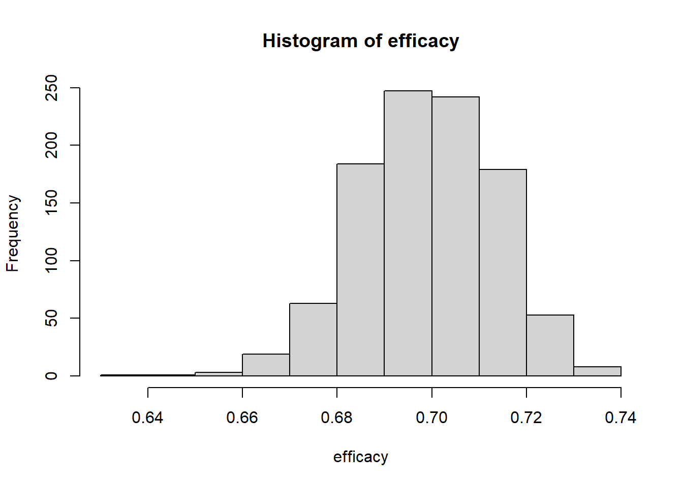

simulations overtime

Tebu

box_time = data.frame()
time = seq(0,10, 1)

b0_decline =-1.518
b0_se_decline =  0.065
b1_decline = 0.147
b1_se_decline = 0.012
n = 30000
for(i in 1:length(time)){
  
y =  rnorm(n, b0_decline,b0_se_decline) + time[i]* rnorm(n,b1_decline,b1_se_decline)  
efficacy = (1-exp(y))
a = data.frame(time = time[i],lambda=efficacy)
box_time = box_time %>% 
  bind_rows(a)
}

# box_time



# box_time %>% 
#   ggplot(aes(time, lambda*100))+
#   geom_point()+
#   labs(y = "Efficacy")+
#   ylim(0,100)

simul_decay = function(data_ef, cost){
# cost = 75
N = n*length(time)
sev_n = rbeta(N, 1.707, 1.266)
sev_f = sev_n*(1-data_ef$lambda) 
normal_correlated<-gera.norm.bid.geral(N,0.21,0,0,1,1)
b0_n = pnorm(normal_correlated[,2])
b1_n = pnorm(normal_correlated[,1])
b0 = qnorm(b0_n, mean_intercept,sd_intercept)
b1 = -qgamma(b1_n, shape, rate,)
rm(b0_n,b1_n,normal_correlated)

# Calculating the alpha coeficient
alfa = (b1/b0)*100

# Calculating yield gain
yn  = b0 - (-alfa*b0*sev_n)
yf  = b0 - (-alfa*b0*sev_f)

soy_price = rnorm(N, mean(sbr_price$price),sd(sbr_price$price))

yield_gain = yf-yn
yield_gain_perc = ((yf - yn)/yn)*100
yield_gain_perc = ((yf/yn)-1)*100
income = yield_gain*soy_price
CP = cost/soy_price
profit = (yield_gain>=CP)
profit_50 = (income>=cost+(cost*0.5))#*1

box_time2 = data_ef %>% 
  mutate(yield_gain) %>% 
  mutate(yield_gain_perc) %>% 
  mutate(income) %>% 
  mutate(CP, cost) %>% 
  mutate(profit,
         profit_50) %>% 
  group_by(time) %>% 
  mutate(P = mean(profit),
         P_50 = mean(profit_50))
return(box_time2)
}

tebu_75 = simul_decay(data_ef = box_time, cost = 75)
tebu_100 = simul_decay(data_ef = box_time, cost = 100)
tebu_125 = simul_decay(data_ef = box_time, cost = 125)
tebu = bind_rows(tebu_75,tebu_100, tebu_125)

tebu %>% 
  group_by(time,cost) %>% 
  slice(1L) %>% 
  pivot_longer(10:11, names_to = "Profits", values_to = "prob") %>% 
  mutate(Profits = case_when(Profits =="P" ~ " Break-even",
                             Profits =="P_50" ~ "50% profit")) %>% 
  ggplot()+
  geom_hline(yintercept = 0.5, color = "gray", size =1, linetype =2)+
  geom_line(aes((time+2004), prob, color = as.factor(cost) ),
            size = 1.2)+
  facet_wrap(~Profits)+
  scale_color_colorblind()+
  labs(y = "Probability of offseting costs",
       x = "Time",
       color = "Cost (US$)")+
  ylim(0,1)+
  theme_minimal_grid()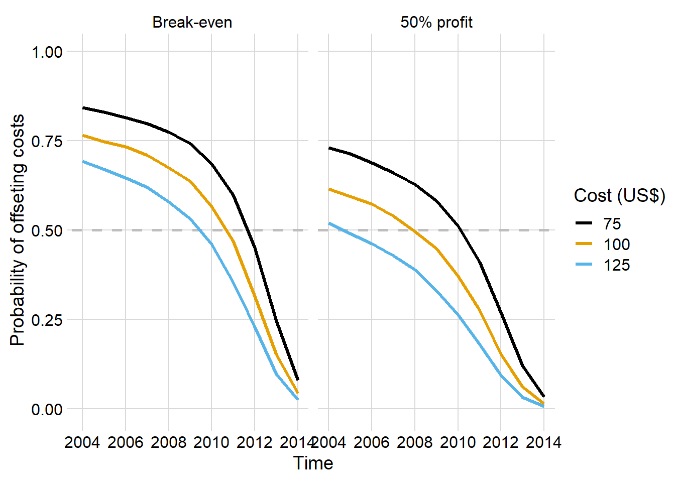

Cypr

box_time_mix = data.frame()
time = seq(0,10, 1)
#mix intercept
# b0_decline =-2.151
# b0_se_decline =  0.121

# tebu intercept
b0_decline =-1.518
b0_se_decline =  0.065

# b1_decline = 0.132
# b1_se_decline = 0.022

b1_decline =0.061
b1_se_decline = 0.015

n = 30000
for(i in 1:length(time)){
  
y =  rnorm(n, b0_decline,b0_se_decline) + time[i]* rnorm(n,b1_decline,b1_se_decline)  
efficacy = (1-exp(y))
a = data.frame(time = time[i],lambda=efficacy)
box_time_mix = box_time_mix %>% 
  bind_rows(a)
}

mix_75 = simul_decay(data_ef =  box_time_mix, cost = 75)
mix_100 = simul_decay(data_ef = box_time_mix, cost = 100)
mix_125 = simul_decay(data_ef = box_time_mix, cost = 125)
mix = bind_rows(mix_75,mix_100, mix_125)

mix %>% 
  group_by(time,cost) %>% 
  slice(1L) %>% 
  pivot_longer(10:11, names_to = "Profits", values_to = "prob") %>% 
  mutate(Profits = case_when(Profits =="P" ~ " Break-even",
                             Profits =="P_50" ~ "50% profit")) %>% 
  ggplot()+
  geom_hline(yintercept = 0.5, color = "gray", size =1, linetype =2)+
  geom_line(aes((time+2004), prob, color = as.factor(cost) ),
            size = 1.2)+
  facet_wrap(~Profits)+  
  scale_color_colorblind()+
  labs(y = "Probability of offseting costs",
       x = "Time",
       color = "Cost (US$)")+
  ylim(0,1)+
  theme_light()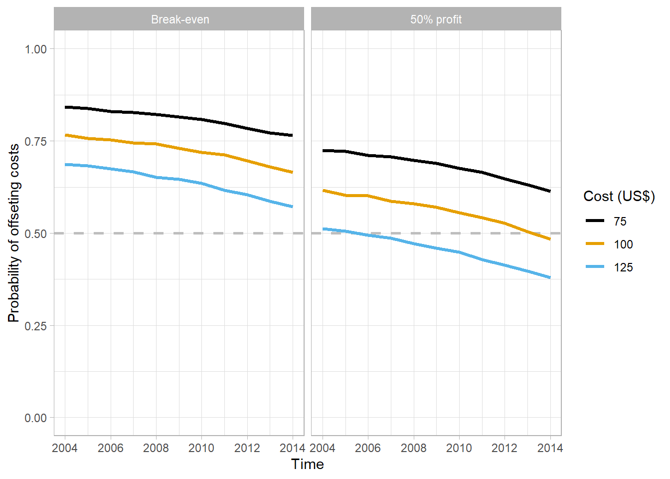

Combo figura

prob_time =  function(data, prof_class){

data %>% 
  group_by(time,cost) %>% 
  slice(1L) %>% 
  pivot_longer(10:11, names_to = "Profits", values_to = "prob") %>% 
  mutate(Profits = case_when(Profits =="P" ~ "Break-even",
                             Profits =="P_50" ~ "50% profit")) %>% 
  filter(Profits == prof_class) %>% 
  ggplot(aes((time), prob))+
    
  annotate("rect",ymin = 0, ymax =0.25, 
            xmin = -5, xmax = 15,
            fill = "#eff3ff",colour="white",
            # alpha = 0.8,
           size = 0.3)+
  annotate("rect",ymin = 0.25, ymax =0.5, 
            xmin = -5, xmax = 15,
            fill = "#bdd7e7",colour="white",
            # alpha = 0.8,
           size = 0.3)+
    annotate("rect",ymin = 0.5, ymax =0.75, 
            xmin = -5, xmax = 15,
            fill = "#6baed6",colour="white",
            # alpha = 0.8,
            size = 0.3)+
    annotate("rect",ymin = 0.75, ymax =1, 
            xmin = -5, xmax = 15,
            fill = "#2171b5", colour="white",
            # alpha = 0.8,
            size = 0.3)+
    
    
  # geom_hline(yintercept = 0.75, color = "gray", size =0.8, linetype =2)+
  geom_step(direction = "hv",size = 1.2,
            aes( color = as.factor(cost) ))+
  scale_x_continuous(breaks = seq(0,10,1))+
  # scale_color_manual(values = c("red" , "#DC143C","darkred"))+
  scale_color_manual(values = c("#fecc5c" , "#fd8d3c","#e31a1c"))+
  # scale_color_manual(values = c("#000000" , "#252525","#525252"))+
  labs(y = "Probability",
       x = "Time (years)",
       color = "Cost (US$/ha)")+
 coord_cartesian(xlim=c(0,10), ylim = c(0,1))+
  theme_light()+
    theme(#panel.grid.major = element_blank()+
          panel.grid =  element_blank())
  
  }

tebu_g1 = prob_time(tebu, prof_class ="Break-even")+
    labs(title = "High annual rate of decline"
         # subtitle = "Offset costs"
         )
tebu_g2 = prob_time(tebu, prof_class ="50% profit")+
    labs(title = "High annual rate of decline",
         subtitle = "50% profit"
         )
mix_g1 = prob_time(mix, prof_class ="Break-even")+
    labs(title = "Low annual rate of decline"
         # subtitle = "Offset costs"
         )
mix_g2 = prob_time(mix, prof_class ="50% profit")+
    labs(title = "Low annual rate of decline",
         subtitle = "50% profit"
         )

tebu_g1+mix_g1+
  plot_layout(guides = "collect")+
  plot_annotation(tag_levels = 'A')&
  theme(legend.position = "bottom",
        plot.title = element_text(size = 10))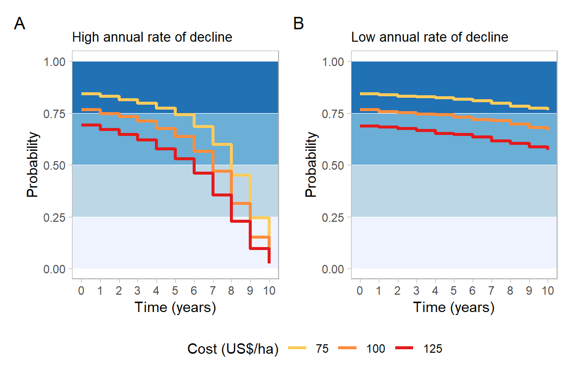

ggsave("figs/prob_time.png", dpi = 600, height = 4, width = 7)
ggsave("figs/prob_time.pdf", dpi = 600, height = 4, width = 7)

Copyright 2017 Emerson Del Ponte