Introduction

This repository contains the code and data processing workflow supporting the analyses presented in the study:
“Quantifying ENSO-mediated shifts in soybean rust impact: Yield loss dynamics and management implications in Brazil.”

Soybean rust (SBR), caused by Phakopsora pachyrhizi, is a major threat to soybean production in Brazil. The study investigates how climate variability, specifically the El Niño Southern Oscillation (ENSO), influences SBR-related yield losses and the performance of disease management strategies. To this end, we analyzed a comprehensive dataset of 417 field trials conducted across 73 locations in Brazil from 2005 to 2020.

The primary goals of the analysis were to:

Estimate disease damage coefficients (i.e., the relationship between disease severity and yield loss) under different ENSO phases (warm, Neutral, cold).
Assess the effectiveness of control measures across these climatic contexts.
Quantify how ENSO conditions modulate both disease impact and management outcomes.

This codebase includes all steps for:

Cleaning and structuring raw trial data
Classifying ENSO phases
Fitting statistical models to estimate damage coefficients
Performing meta-analyses and producing summary figures and tables

Getting started

This project uses renv to manage package dependencies and ensure reproducible computational environments. Follow the steps below to set up and execute the code.

Prerequisites

R (≥ 4.4.1) Ensure you have a compatible version of R installed. You can download R from CRAN.
Git (optional but recommended) To clone the repository, install Git from git-scm.com. Alternatively, you can download the repository as a ZIP.
Project Files

Steps to Initialize the Environment

Clone or Download the Repository

git clone https://github.com/AlvesKS/paper_ENSO_SBR_damage.git
cd your-repo

Alternatively, you can download the repository as a ZIP file and extract it to your working directory using the code below:

download.file("https://github.com/AlvesKS/paper_ENSO_SBR_damage/archive/refs/heads/main.zip", destfile = "paper-white-mold-prediction-modeling.zip", mode = "wb")

unzip("paper-white-mold-prediction-modeling.zip", list = FALSE)

Open the Project in R

The repository files should be inside the paper-white-mold-prediction-modeling/ directory, which should be locatated in your working directory. Open the file .Rproj file.

Install or update the renv package (if not already installed)

If you haven’t installed renv yet, run the following command in your R console. If you already have renv, ensure it is updated to the latest version.

install.packages("renv")

Restore the Project Library

This command reads the renv.lock file and installs the exact package versions into a project-specific library (renv/library/).
If prompted to update renv itself, follow the message and restart R afterward.

renv::restore()

Verify Successful Restoration

After renv::restore() completes, you should see messages indicating that required packages were installed. You can check the status with:

renv::status()

If all dependencies are up to date, renv::status() will report no divergences from the lockfile.

Running the Analysis

Locate the Main Script

The primary analysis script are located in the R/ directory named as main_damage_coef.qmd.

Execute the Workflow

From now on, you can run the analysis by executing the code chunks in the R quarto file. The code is organized into sections, and you should each execute section sequentialy or knit the entire document to generate a report.

Inspect and Export Outputs

Output figures (PNG/PDF) are saved in the figs/ folder.

Packages

library(tidyverse)
library(gsheet)
library(cowplot)
library(patchwork)
library(lemon)
library(lme4)
library(ggforce)
library(ggrepel)
library(lmerTest)
library(emmeans)
library(multcomp)
library(ggthemes)
library(metafor)
library(minpack.lm)

theme_set(theme_half_open(font_size = 10))

Data

Soybean Rust data

data_load = read.csv("data/raw-data-2005-2020.csv") |> 
  mutate(sev = as.numeric(sev),
         yld = as.numeric(yld))

Warning: There were 2 warnings in `mutate()`.
The first warning was:
ℹ In argument: `sev = as.numeric(sev)`.
Caused by warning:
! NAs introduzidos por coerção
ℹ Run `dplyr::last_dplyr_warnings()` to see the 1 remaining warning.

ENSO data

enso_data = read.csv("data/enso.csv")

Classifying the years based on Oceanic Niño Index (ONI) on the October, November, and December (OND) trimester. Seasons with ONI higher then 75 percentiles were classified as warm, year with ONI lower then its 25 percentiles were classified as Cold, and the years with ONI within the 25 and 75 percentiles were classified as neutral.

enso_data_class = enso_data |> 
  mutate(year = as.character(Year+1)) |> 
  dplyr::select(-Year) |> 
  mutate(selected_trimester = OND) |> 
  dplyr::select(selected_trimester, year) |> 
  filter(!is.na(selected_trimester),
         year != 2021) |> 
  mutate(quantile_0.75 = quantile(selected_trimester, 0.75),
         quantile_0.25 = quantile(selected_trimester, 0.25)) |>
  mutate(enso = case_when(selected_trimester > quantile_0.75 ~ "Warm",
                          selected_trimester <=quantile_0.25 ~ "Cold",
                          selected_trimester <= quantile_0.75 & selected_trimester > quantile_0.25 ~ "Neutral"),
         year = as.numeric(year))
enso_data_class

enso_data_class |> 
  summarise(quantile_0.75 = unique(quantile_0.75),
            quantile_0.25 = unique(quantile_0.25))

enso_gg = enso_data_class|> 
  mutate(enso = factor(enso, levels = c("Neutral", "Warm", "Cold")))|> 
  ggplot(aes( as.factor(year),selected_trimester,  color = enso))+
  geom_hline(yintercept = 0)+
  geom_hline(yintercept = c(-0.725,0.75), linetype = 2, color = "gray")+
  geom_errorbar(aes(ymin=0, ymax  = selected_trimester), width = 0, color = "black")+
  geom_point(size = 3)+
  
  scale_color_colorblind()+
  theme_half_open(font_size = 12)+
  scale_y_continuous(breaks = seq(-3,3,by = 0.75), limits = c(-3,3))+
  theme(axis.text.x = element_text(angle = 45, hjust = 1),
        # legend.position = "top",
        strip.background = element_blank())+
  labs(x = "Crop Season",
       y = "Oceanic Niño Index",
       color = "ENSO phase (OND)")
enso_gg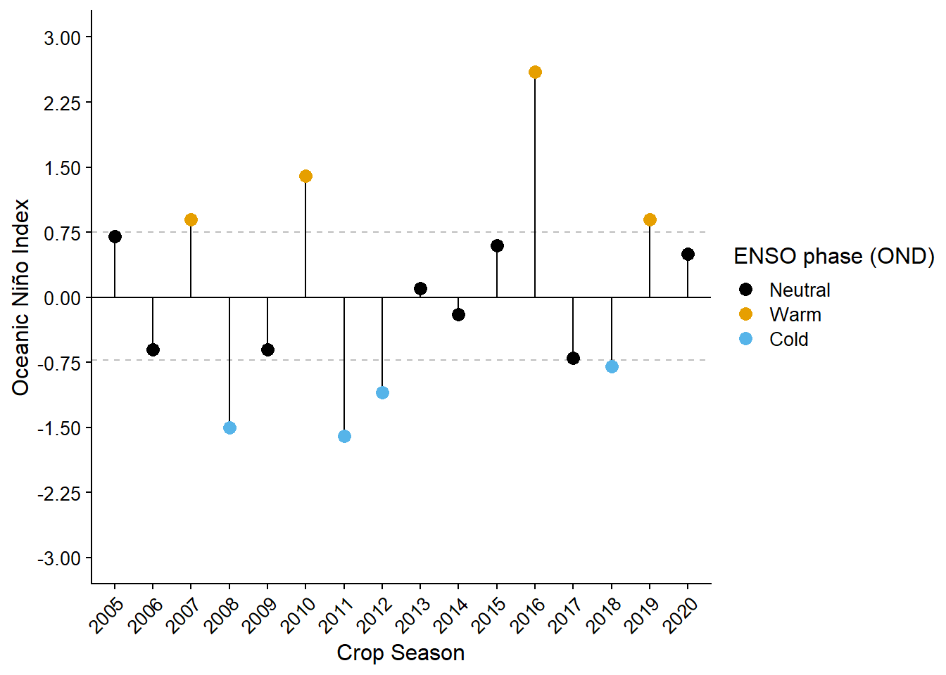

ggsave("figs/ONI_OND.png", dpi = 600, height = 4, width = 7, bg = "white")

Counting the number of year for each phase

enso_data_class |> 
  count(enso)

Data wrangling

data_load2 = data_load |> 
  mutate(sev = as.numeric(sev)) |> 
  full_join(enso_data_class) |> 
  mutate(enso = factor(enso, levels = c("Neutral", "Warm", "Cold"))) |> 
  filter(!is.na(sev),
         !is.na(yld)) |> 
  mutate(study = as.factor(study)) |> 
  mutate(region = case_when(state %in% c("SP","BA","MG", "MS", "MT", "GO",  "MA", "DF", "TO")~"North",
                             state %in% c("RS","SC","PR") ~"South"),
         region =factor(region, levels = c("South","North"))) |> 
  group_by(study) |> 
  mutate(difer = max(sev) - min(sev)) |> 
  filter(difer>5)

Joining with `by = join_by(year)`

data_load2 |> 
  filter(active_ingred == "CHECK") |> 
  ggplot(aes(sev, difer))+
  geom_point(color = "black", size =2, shape =1)+
  geom_hline(yintercept = 5, linetype = "dashed", color = "gray", size = 1.2)+
  geom_abline(slope = 1, intercept = 0, color = "darkred", size = 1.4)+
  annotate("text",x = 100, y = 5, label = "Minimum difference = 5 p.p", vjust = -1, hjust = 1)+
  coord_cartesian(xlim = c(0,100),
                  ylim = c(0,100))

Warning: Using `size` aesthetic for lines was deprecated in ggplot2 3.4.0.
ℹ Please use `linewidth` instead.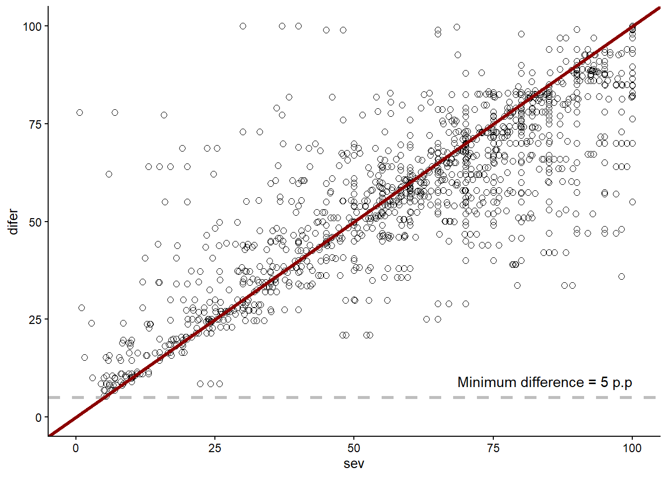

unique(data_load2$state)

 [1] "BA" "PR" "MG" "MS" "MT" "GO" "SP" "MA" "DF" "TO" "RS" "SC"

length(unique(data_load2$state))

[1] 12

data_load2 |> 
  group_by(state) |> 
  summarise(n_loc = length(unique(location))) |> 
  summarise(sum(n_loc))

length(unique(data_load2$year))

[1] 16

data_load2 |> 
  group_by(enso) |> 
  summarise(n_study = length(unique(study)),
            n_year = length(unique(year)),
            n_loc = length(unique(location)),
            n_state = length(unique(state)))

Tranformations

Converting percent severity into proportion and calculating logits

only_check_df = data_load2 |> 
  filter(active_ingred == "CHECK") |> 
  mutate(sev = case_when(sev == 100 ~ 99.9,
                         sev == 0 ~ 0.1,
                         sev>0 & sev<100 ~ sev), 
           logit_sev =  DescTools::Logit(sev/100))

Exploratory analysis

Average, min and max severity

Overal

 data_load2 |> 
  filter(active_ingred == "CHECK") |> 
  ungroup() |> 
  summarise(avg_sev = mean(sev),
            max_sev = max(sev),
            min_sev = min(sev))

by year

 data_load2 |> 
  filter(active_ingred == "CHECK") |> 
  group_by(year) |> 
  summarise(avg_sev = mean(sev),
            max_sev = max(sev),
            min_sev = min(sev)) |> 
  arrange(max_sev)

By ENSO state

 data_load2 |> 
  filter(active_ingred == "CHECK") |> 
  group_by(enso) |> 
  summarise(avg_sev = mean(sev),
            max_sev = max(sev),
            min_sev = min(sev))

plot

enso_sev_gg = data_load2 |> 
  filter(active_ingred == "CHECK") |> 
  ggplot(aes(enso, sev, color = enso))+
  geom_sina(color = "gray")+
  geom_boxplot(fill= NA, size = 1)+
  theme_half_open(font_size = 12)+
  scale_color_colorblind()+
  labs( y = "",
        x = "",
        color = "",
        title = "")
enso_sev_gg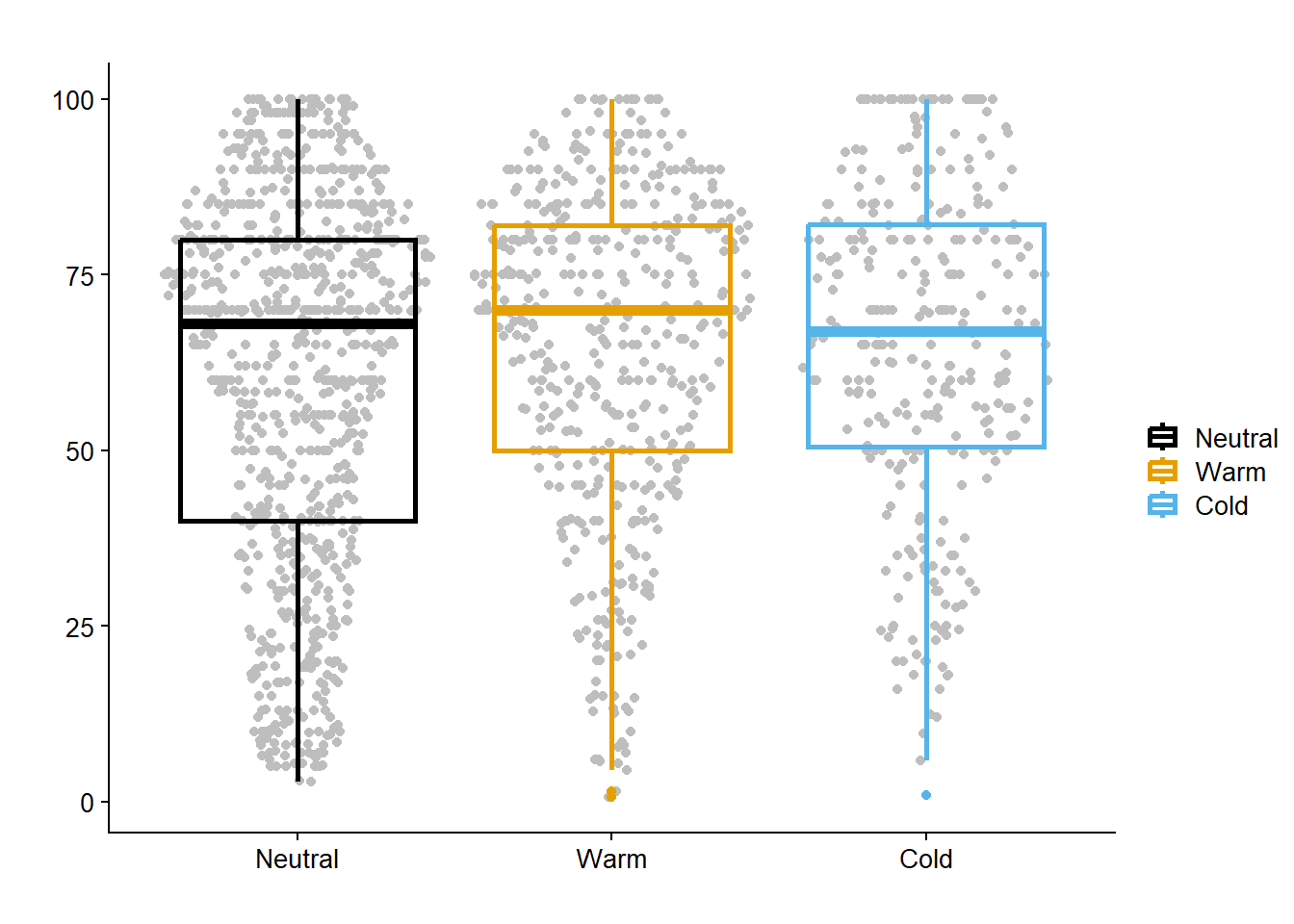

Graph over time

sev_untreat_gg = only_check_df |> 
  ggplot(aes(as.factor(year),  sev, color = enso))+
  geom_sina(color = "gray80")+
  geom_boxplot(fill =NA, size = 1, outlier.color = NA)+
  labs( y = "Severity (%)",
        x = "",
        color = "",
        title = " ")+
  theme_half_open(font_size = 12)+
  # facet_wrap(~region)+
  scale_color_colorblind()
sev_untreat_gg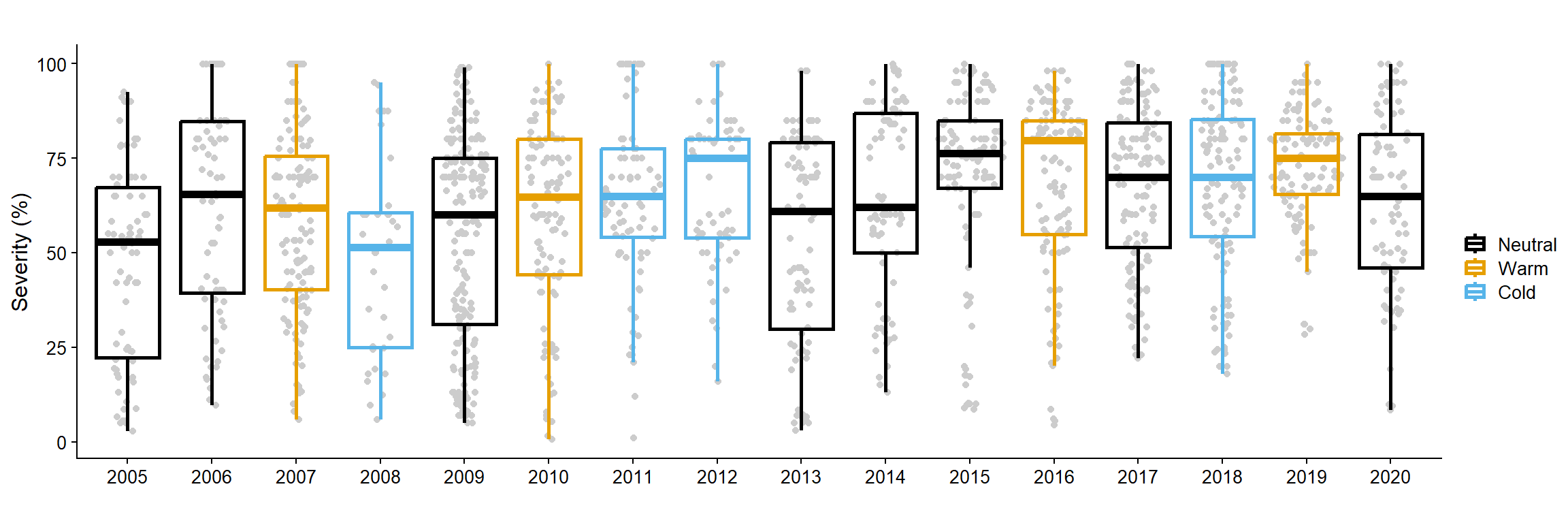

Average, min and max yield

Overal

 data_load2 |> 
  filter(active_ingred == "CHECK") |> 
  ungroup() |> 
  summarise(avg_yld = mean(yld),
            max_yld = max(yld),
            min_yld = min(yld))

by year

 data_load2 |> 
  filter(active_ingred == "CHECK") |> 
  group_by(year) |> 
  summarise(avg_yld = mean(yld),
            max_yld = max(yld),
            min_yld = min(yld)) |> 
  arrange(avg_yld)

By ENSO state

 data_load2 |> 
  filter(active_ingred == "CHECK") |> 
  group_by(enso)|> 
  summarise(avg_yld = mean(yld),
            max_yld = max(yld),
            min_yld = min(yld)) |> 
  arrange(avg_yld)

Modeling Severity (untreated) and ENSO

Mixed-effect model

model_check = lmer(logit_sev ~ enso+ (1|year/study), data = only_check_df,REML = F)

Model summary

summary(model_check)

Linear mixed model fit by maximum likelihood . t-tests use Satterthwaite's
  method [lmerModLmerTest]
Formula: logit_sev ~ enso + (1 | year/study)
   Data: only_check_df

     AIC      BIC   logLik deviance df.resid 
  4506.7   4539.3  -2247.3   4494.7     1680 

Scaled residuals: 
    Min      1Q  Median      3Q     Max 
-7.5458 -0.2094  0.0000  0.2012  9.5043 

Random effects:
 Groups     Name        Variance Std.Dev.
 study:year (Intercept) 2.80243  1.6740  
 year       (Intercept) 0.07201  0.2683  
 Residual               0.35208  0.5934  
Number of obs: 1686, groups:  study:year, 418; year, 16

Fixed effects:
            Estimate Std. Error      df t value Pr(>|t|)    
(Intercept)   0.6678     0.1523 13.0217   4.385 0.000735 ***
ensoWarm      0.2028     0.2544 11.8761   0.797 0.441117    
ensoCold      0.4745     0.2843 16.4863   1.669 0.113967    
---
Signif. codes:  0 '***' 0.001 '**' 0.01 '*' 0.05 '.' 0.1 ' ' 1

Correlation of Fixed Effects:
         (Intr) ensWrm
ensoWarm -0.599       
ensoCold -0.536  0.321

Pairwise comparison

pairs(emmeans(model_check, ~enso))

 contrast       estimate    SE   df t.ratio p.value
 Neutral - Warm   -0.203 0.290 18.6  -0.699  0.7671
 Neutral - Cold   -0.474 0.320 23.0  -1.485  0.3165
 Warm - Cold      -0.272 0.355 21.4  -0.764  0.7283

Degrees-of-freedom method: kenward-roger 
P value adjustment: tukey method for comparing a family of 3 estimates

All Severity data (plot)

sev_gg = data_load2 |> 
  ggplot(aes(as.factor(year),  sev, color = enso))+
  geom_sina(color = "gray80")+
  geom_boxplot(fill =NA, size = 1, outlier.color = NA)+
  labs( y = "Severity (%)",
        x = "Growing season",
        color = "",
        title = "Data from all plots")+
  theme_half_open(font_size = 12)+
  # facet_wrap(~region)+
  scale_color_colorblind()
sev_gg

Modeling soybean yield and ENSO

enso_yld_gg = data_load2 |> 
  filter(active_ingred == "CHECK") |> 
  ggplot(aes(enso, yld, color = enso))+
  geom_sina(color = "gray")+
  geom_boxplot(fill= NA, size = 1)+
  scale_color_colorblind()+
  theme_half_open(font_size = 12)+
  labs( y = "",
        x = "",
        color = "",
        title = "")
enso_yld_gg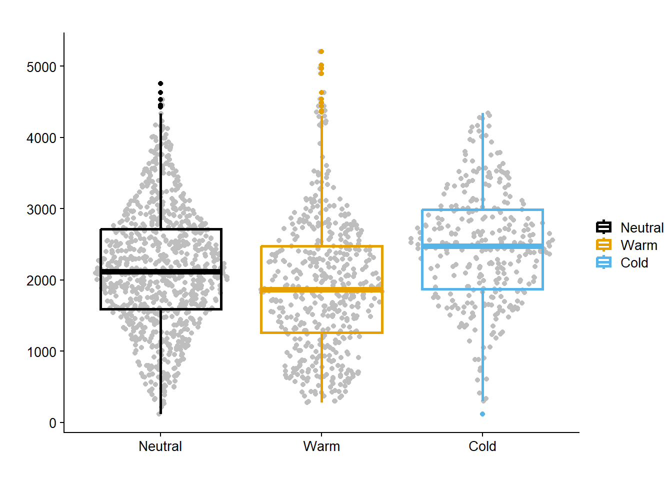

Graph over time

yld_untreat_gg = data_load2 |> 
  filter(active_ingred == "CHECK")|> 
  ggplot(aes(as.factor(year),  yld, color = enso))+
  geom_sina(color = "gray80")+
  geom_boxplot(size =1, fill = NA, outlier.colour = NA)+
  labs( y = "Yield (kg/ha)",
        x = "Growing season",
        color = "",
        title = "")+
  theme_half_open(font_size = 12)+
  scale_color_colorblind()
yld_untreat_gg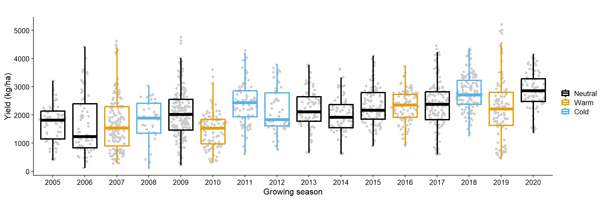

Mixed-effect model

model_check_yld = lmer(yld ~ enso + (1|year/study), data = only_check_df, REML = F)

Model summary

summary(model_check_yld)

Linear mixed model fit by maximum likelihood . t-tests use Satterthwaite's
  method [lmerModLmerTest]
Formula: yld ~ enso + (1 | year/study)
   Data: only_check_df

     AIC      BIC   logLik deviance df.resid 
 24878.7  24911.3 -12433.4  24866.7     1680 

Scaled residuals: 
    Min      1Q  Median      3Q     Max 
-4.5778 -0.4421  0.0067  0.4548  5.2378 

Random effects:
 Groups     Name        Variance Std.Dev.
 study:year (Intercept) 618988   786.8   
 year       (Intercept)  96443   310.6   
 Residual                57242   239.3   
Number of obs: 1686, groups:  study:year, 418; year, 16

Fixed effects:
            Estimate Std. Error      df t value Pr(>|t|)    
(Intercept)  2148.18     123.74   14.70  17.361 3.36e-11 ***
ensoWarm     -219.25     211.23   13.94  -1.038    0.317    
ensoCold      181.70     221.18   16.40   0.822    0.423    
---
Signif. codes:  0 '***' 0.001 '**' 0.01 '*' 0.05 '.' 0.1 ' ' 1

Correlation of Fixed Effects:
         (Intr) ensWrm
ensoWarm -0.586       
ensoCold -0.559  0.328

Pairwise comparison

cld(emmeans(model_check_yld, ~enso))

All yield data

Graph over time

yld_gg = data_load2 |> 
  ggplot(aes(as.factor(year),  yld, color = enso))+
  geom_sina(color = "gray80")+
  geom_boxplot(size =1, fill = NA, outlier.colour = NA)+
  labs( y = "Yield (kg/ha)",
        x = "Growing season",
        color = "",
        title = "Data from all plots")+
  theme_half_open(font_size = 12)+
  scale_color_colorblind()
yld_gg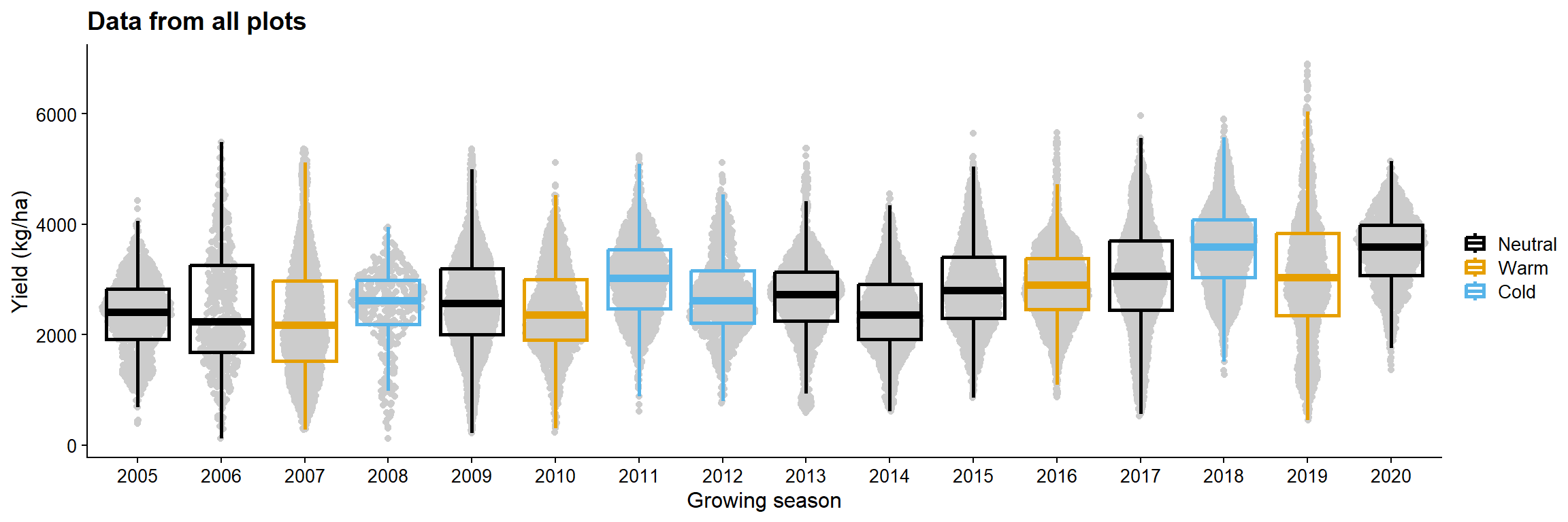

Combo plot

sev_untreat_gg + enso_sev_gg+
  yld_untreat_gg +enso_yld_gg+
  plot_annotation(tag_levels = "a")+
  plot_layout(ncol = 2,
              widths = c(1,0.25),
              guides = "collect")&
  theme(axis.text = element_text(size =8))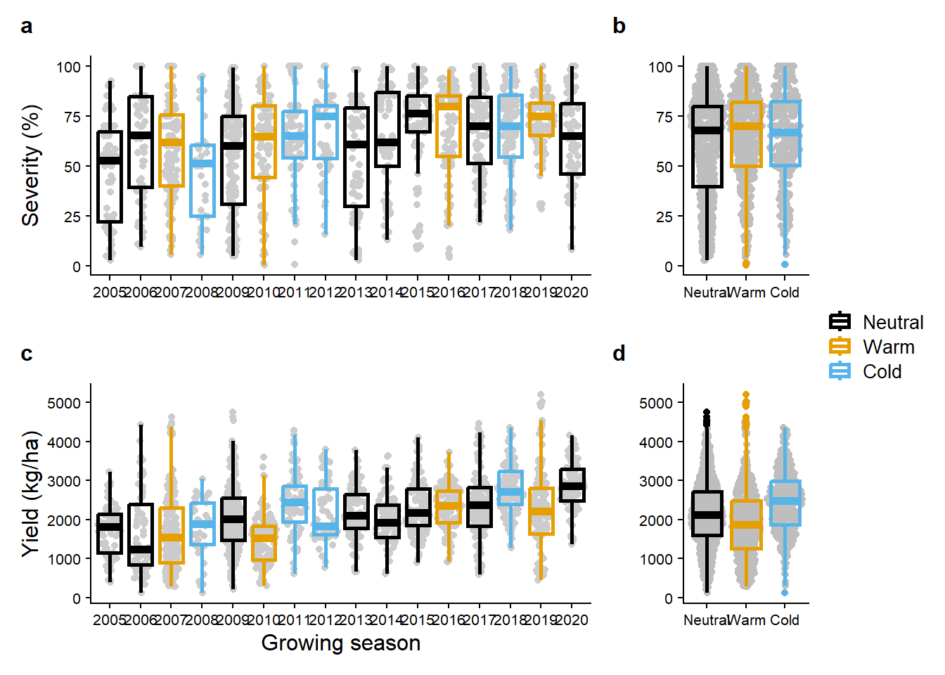

ggsave("figs/data_over_time.png", dpi = 600, height = 6, width = 9, bg = "white")
ggsave("figs/data_over_time.pdf", dpi = 600, height = 6, width = 9, bg = "white")

Modeling disease damage

Yield vs. Severity

data_load2 |> 
  ggplot(aes(sev, yld, color = enso))+
  # geom_point(alpha = 0.1)+
  geom_smooth(aes(group=study),
              method = "lm", size =0.1,se = F, fullrange   =T)+
  geom_smooth(aes(group = enso),  color = "red", se = F, method = "lm")+
  scale_color_colorblind()+
  theme_half_open()+
  facet_rep_grid(~enso)+
  ylim(0,7500)+
  labs(x = "Severity (%)",
       y = "Yield (kg/ha)",
       color = "")+
  theme(strip.background = element_blank())

`geom_smooth()` using formula = 'y ~ x'
`geom_smooth()` using formula = 'y ~ x'

Warning: Removed 1124 rows containing missing values or values outside the scale range
(`geom_smooth()`).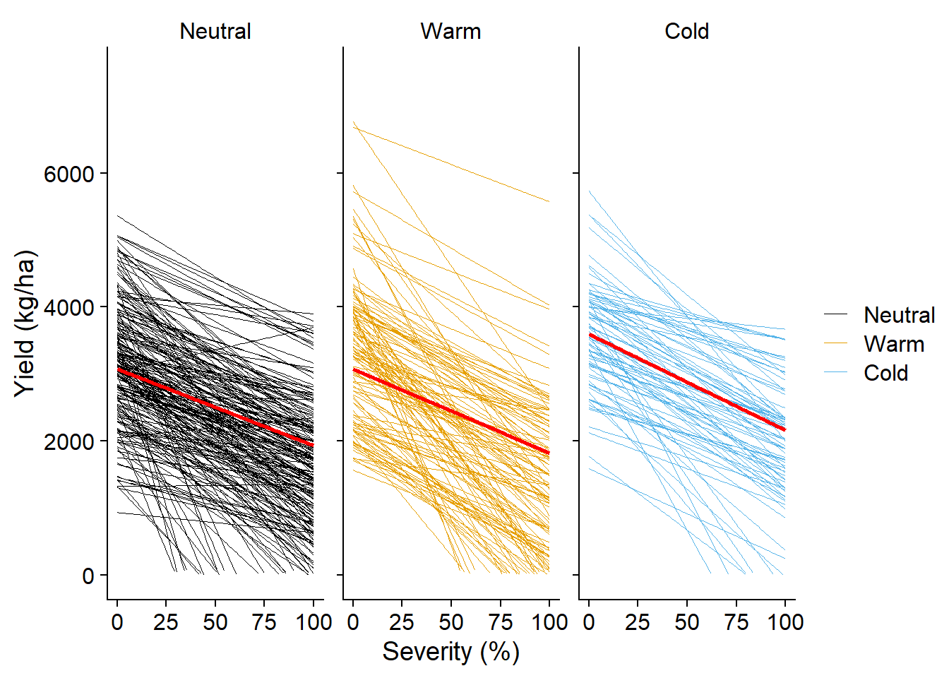

Meta-analysis

Ordinary Regression

reg_dc = data_load2 |> 
  group_by(study, year, region, enso) |> 
  summarise(intercept = lm(yld~sev)$coefficients[1],
            slope = lm(yld~sev)$coefficients[2],
            r2 = summary(lm(yld~sev))$r.squared,
            sigma = summary(lm(yld~sev))$sigma) %>%
  mutate(Dc = (slope/intercept)*100) |> 
  filter(Dc<0.5)

`summarise()` has grouped output by 'study', 'year', 'region'. You can override
using the `.groups` argument.

reg_dc

Graph of the regression lines

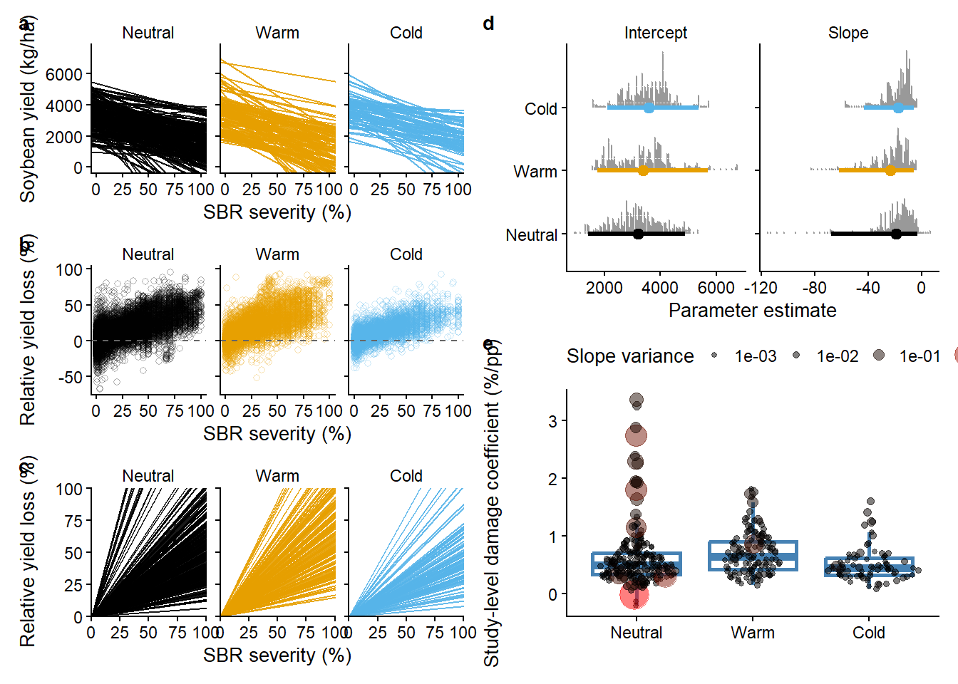
reg1_gg = reg_dc |> 
  ggplot()+
  geom_abline(aes(intercept = intercept, slope = slope, color= enso), alpha = 0.9)+
  labs(x = "Severity (%)",
       y = "Yield (kg/ha)")+
  theme_half_open()+
  xlim(0,100)+
  ylim(0,7500)+
  scale_color_colorblind()+
  theme_half_open(font_size = 10)+
  facet_rep_grid(~enso)+
  labs(x = "SBR severity (%)",
       y = "Soybean yield (kg/ha)",
       color = "")+
  theme(strip.background = element_blank(),
        legend.position = "none")
reg1_gg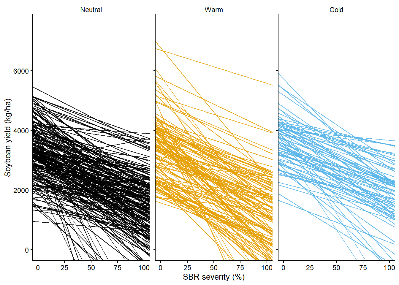

Distribution of intercepts and slopes

reg_dc |> 
  pivot_longer(c(intercept, slope), names_to = "par",values_to = "par_value")

reg_dc |> 
  pivot_longer(c(intercept, slope), names_to = "par",values_to = "par_value") |> 
  group_by(par, enso) |> 
  summarise(avg = round(mean(par_value),1),
            std_dev = round(sd(par_value),1),
            q_lw = round(quantile(par_value,c(0.025)),1),
            q_up = round(quantile(par_value,c(0.975)),1),
            q_up-q_lw)

`summarise()` has grouped output by 'par'. You can override using the `.groups`
argument.

parms_gg = reg_dc |> 
  pivot_longer(c(intercept, slope), names_to = "par",values_to = "par_value") |>
  mutate(par = ifelse(par=="intercept", "Intercept", "Slope")) |> 
  ggplot(aes(y = enso, par_value,color = enso))+
  ggdist::stat_dotsinterval(slab_shape = 19,point_interval = "mean_qi", .width = c(0.95), quantiles = 500, slab_color= "gray60") +
  scale_color_colorblind()+
  theme_half_open(font_size = 10)+
  labs(x = "Parameter estimate",
       y = "")+
  facet_rep_grid(~par, scales = "free")+
  theme(strip.background = element_blank(),
        legend.position = "none")
parms_gg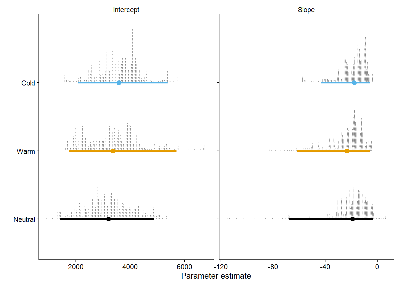

Relative yield loss (%) relative to β₀

data2 = data_load2 |> 
  full_join(reg_dc) |> 
  mutate(l = 100*((intercept - yld)/intercept)) |> 
  filter(!is.na(l))

Joining with `by = join_by(study, year, enso, region)`

data2

data2 |> 
  ggplot(aes(l))+
  geom_histogram(color = "white", bins = 10)&
  theme_half_open()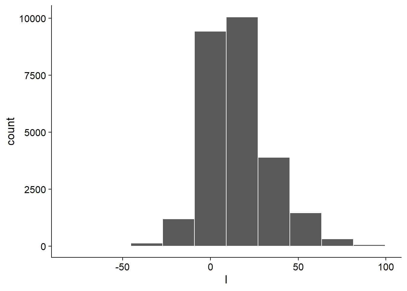

l_gg = data2 |> 
  ggplot(aes(sev,l,color =enso))+
  geom_point( shape =1, alpha = 0.3)+
  # color = "gray80",
  # geom_smooth(method ="lm", 
  #             aes(color =enso),
  #             color = "gray90",
  #             formula = y~0+x)+
  geom_hline(yintercept = 0, linetype = "dashed", color = "gray40")+
  scale_color_colorblind()+
  labs(x = "Severity (%)",
       y = expression("Yield loss relative to "~β[0]))+
  theme_half_open(font_size = 10)+
  facet_rep_grid(~enso)+
  labs(x = "SBR severity (%)",
       # y = expression("Yield loss relative to "~β[0]~"(%)"),
       y = expression("Relative yield loss (%)"),
       color = "")+
  theme(strip.background = element_blank(),
        legend.position = "none")
l_gg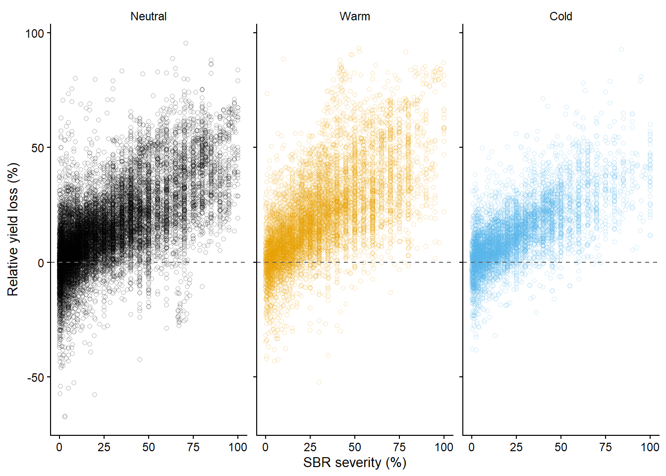

Second Regression l ~ 0 + sev

data3 = data2 |> 
  group_by(study, year, enso, region) |> 
  summarise(slope = lm(l~0+sev)$coefficients,
            vi = as.numeric(vcov(lm(l~0+sev)))
            ) |> 
  full_join(enso_data_class)

`summarise()` has grouped output by 'study', 'year', 'enso'. You can override
using the `.groups` argument.
Joining with `by = join_by(year, enso)`

data3

reg2_gg =
  data3 |> 
  mutate(enso = factor(enso, levels = c("Neutral", "Warm", "Cold"))) |> 
  ggplot()+
  geom_abline(aes(intercept = 0, slope = slope, color= enso), alpha = 0.9)+
  labs(x = "Severity (%)",
       y = "Yield (kg/ha)")+
  theme_half_open()+
  xlim(0,100)+
  ylim(0,100)+
  scale_x_continuous(expand = c(0, 0),
                     limits = c(0,100)) +
  scale_y_continuous(expand = c(0, 0),
                     limits = c(0,100))+
  scale_color_colorblind()+
  theme_half_open(font_size = 10)+
  facet_rep_grid(~enso)+
  labs(x = "SBR severity (%)",
       y = expression("Relative yield loss (%)"),
       color = "")+
  theme(strip.background = element_blank(),
        legend.position = "none")

Scale for x is already present.
Adding another scale for x, which will replace the existing scale.
Scale for y is already present.
Adding another scale for y, which will replace the existing scale.

reg2_gg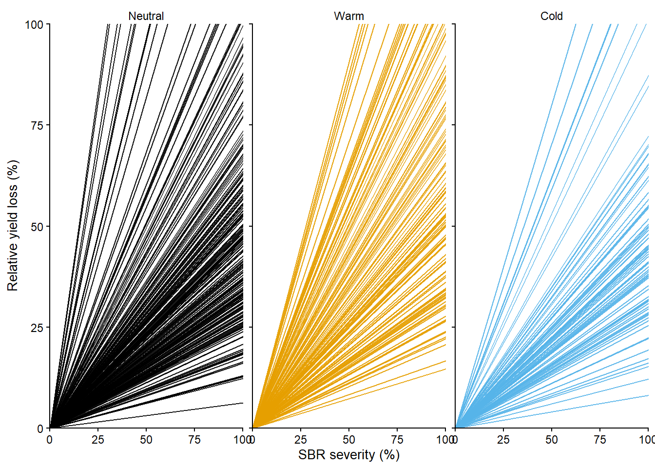

data3 |> 
  group_by(enso) |> 
  summarise(mean(slope),
            median(slope),
            round(quantile(vi,0.95),2))

Damage vs. ENSO phases

data3 |> 
  ggplot(aes(slope))+
  geom_histogram(color = "gray")+
  facet_rep_wrap(~enso, ncol=1 )

`stat_bin()` using `bins = 30`. Pick better value with `binwidth`.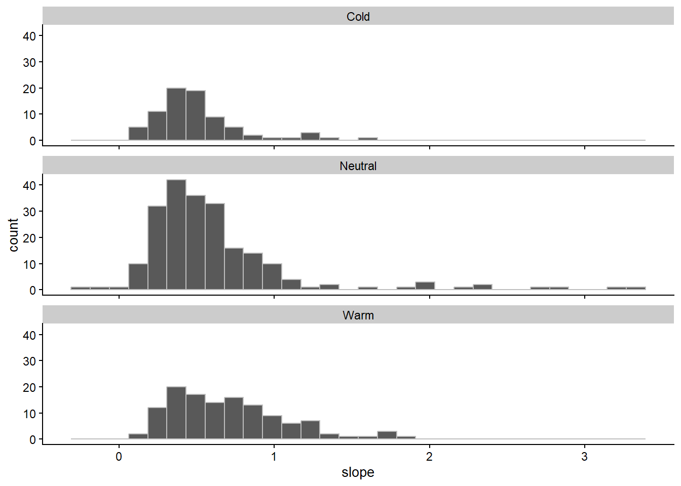

library(scales)


Anexando pacote: 'scales'

O seguinte objeto é mascarado por 'package:purrr':

    discard

O seguinte objeto é mascarado por 'package:readr':

    col_factor

slopes_gg = data3 |> 
  mutate(enso = factor(enso, levels = c("Neutral", "Warm", "Cold"))) |> 
  arrange(slope) |> 
  ggplot(aes(enso, slope ))+
  geom_boxplot(fill = NA, color = "steelblue", size =1, outlier.colour = NA)+
  geom_sina(aes(size = vi, color= vi), alpha = 0.5)+
  scale_size_continuous(range = c(1, 7),
                        #limits =  c(0.01,1),
                        breaks = c(0.001, 0.01, 0.1, 1),
                       label=scientific_format())+
  scale_color_gradient(low = "black",
                       high = "red",
                       #limits = c(0.01, 1), 
                        breaks = c(0.001, 0.01, 0.1, 1),
                       label=scientific_format())+
  guides(color= guide_legend(), 
         size=guide_legend())+
  theme_half_open(font_size = 10)+
  labs(y = "Study-level damage coefficient (%/pp)",
       x = "",
       size = "Slope variance",
       color  = "Slope variance" )+
  theme(legend.position = "top")
slopes_gg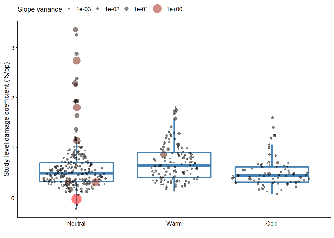

Combo plot

layout <- "
AAAACC
BBBBCC
"

layout <- "
AAAADD
BBBBDD
CCCCDD
"
layout <- "
AAAABBB
CCCCEEE
DDDDEEE
"

layout <- "
AAAABBB
AAAABBB
AAAABBB
CCCCBBB
CCCCEEE
DDDDEEE
DDDDEEE
DDDDEEE
"



# (reg1_gg+parms_gg+l_gg+reg2_gg+slopes_gg)+
((reg1_gg/l_gg/reg2_gg) | (parms_gg/slopes_gg))+
  plot_annotation(tag_levels = 'a')&
  theme(axis.title = element_text(size = 10)
        # plot.tag = element_text(size = 8)
        )

ggsave("figs/regression_lines.png", dpi = 600, width = 10, height = 6, bg ="white")
ggsave("figs/regression_lines.pdf", dpi = 600, width = 10, height = 6, bg ="white")

Meta-analytical model

data4 = data3 |> 
  mutate(year = as.factor(year),
         enso = factor(enso, levels = c("Neutral", "Cold", "Warm")))
metamodel2 = rma.uni(yi = slope,
                    vi = vi,
                    mods = ~ enso, 
                    random = list(~1|year/study),
                    # struct = "HCS",
                    method = "ML",
                    data =data4)

Warning: Extra argument ('random') disregarded.

metamodel2


Mixed-Effects Model (k = 417; tau^2 estimator: ML)

tau^2 (estimated amount of residual heterogeneity):     0.1099 (SE = 0.0080)
tau (square root of estimated tau^2 value):             0.3316
I^2 (residual heterogeneity / unaccounted variability): 99.54%
H^2 (unaccounted variability / sampling variability):   219.29
R^2 (amount of heterogeneity accounted for):            5.61%

Test for Residual Heterogeneity:
QE(df = 414) = 41096.3735, p-val < .0001

Test of Moderators (coefficients 2:3):
QM(df = 2) = 17.5026, p-val = 0.0002

Model Results:

          estimate      se     zval    pval    ci.lb   ci.ub      
intrcpt     0.5651  0.0236  23.9141  <.0001   0.5188  0.6114  *** 
ensoCold   -0.0640  0.0449  -1.4237  0.1545  -0.1520  0.0241      
ensoWarm    0.1258  0.0385   3.2649  0.0011   0.0503  0.2014   ** 

---
Signif. codes:  0 '***' 0.001 '**' 0.01 '*' 0.05 '.' 0.1 ' ' 1

data4 = data3 |> mutate(year = as.factor(year))
metamodel2 = rma.uni(yi = slope,
                    vi = vi,
                    mods = ~ 0+enso, 
                    random = list(~1|year/study),
                    # struct = "HCS",
                    method = "ML",
                    data =data4)

Warning: Extra argument ('random') disregarded.

metamodel2


Mixed-Effects Model (k = 417; tau^2 estimator: ML)

tau^2 (estimated amount of residual heterogeneity):     0.1099 (SE = 0.0080)
tau (square root of estimated tau^2 value):             0.3316
I^2 (residual heterogeneity / unaccounted variability): 99.54%
H^2 (unaccounted variability / sampling variability):   219.29

Test for Residual Heterogeneity:
QE(df = 414) = 41096.3735, p-val < .0001

Test of Moderators (coefficients 1:3):
QM(df = 3) = 1258.6134, p-val < .0001

Model Results:

             estimate      se     zval    pval   ci.lb   ci.ub      
ensoCold       0.5011  0.0382  13.1116  <.0001  0.4262  0.5760  *** 
ensoNeutral    0.5651  0.0236  23.9141  <.0001  0.5188  0.6114  *** 
ensoWarm       0.6909  0.0305  22.6896  <.0001  0.6312  0.7506  *** 

---
Signif. codes:  0 '***' 0.001 '**' 0.01 '*' 0.05 '.' 0.1 ' ' 1

Estimates for each moderator

grid = qdrg(object = metamodel2,  data = data4, at = list(vi = 0, year.c = 0))
# cld(emmeans(grid,specs = ~enso, by = "region"), Letters = letters)
cld(emmeans(grid, specs = ~enso), Letters = letters)

# grid@V

Graphs

Forest plot

forest_gg = data3 |> 
  mutate(study = as.character(study),
         sd = sqrt(vi),
         
         cil = slope - 1.96*sd,
         ciu = slope + 1.96*sd) |> 
  full_join(as.data.frame(emmeans(grid,specs = ~enso))) |> 
  mutate(enso = factor(enso, levels = c("Neutral",  "Warm","Cold"))) |> 
  ggplot(aes(slope,reorder(study, slope),  color= enso))+
  geom_point(size=0.3)+
  geom_errorbar(aes(xmin=cil, xmax = ciu), width = 0,size=0.3, alpha =0.5)+
  geom_vline(xintercept = 0, linetype = "dashed")+
  geom_vline(aes(xintercept = emmean), color = "gray40", size = .5)+
  scale_color_colorblind()+
  facet_rep_wrap(~enso,  scales="free_y")+
  labs(y = "",
       x = "Damage coefficient (%/p.p.)",
       color = "")+
  guides(color = guide_legend(override.aes = list(size=2.5)))+
  theme(axis.text.y = element_blank(),
        axis.ticks.length.y = unit(0, "cm"),
        strip.background = element_blank(),
        legend.position = "bottom")

Joining with `by = join_by(enso)`

forest_gg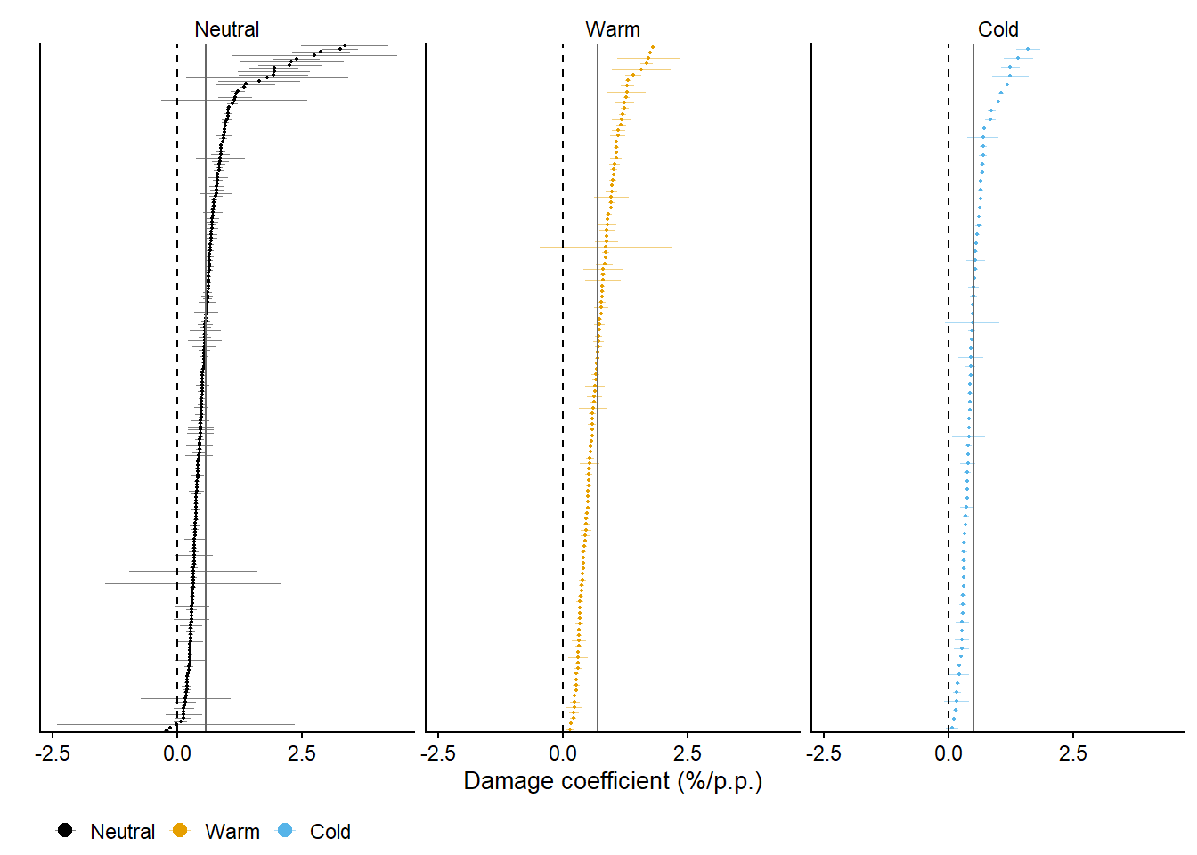

Damage coefficient

dc_data =  as.data.frame(emmeans(grid, specs = ~enso))
dc_data

DC_gg = as.data.frame(emmeans(grid,specs = ~enso)) |> 
    mutate(enso = factor(enso, levels = c("Neutral",  "Warm","Cold"))) |> 
  ggplot(aes(reorder(enso,emmean), emmean, color = enso))+
  geom_point(position = position_dodge(width = 0.2), size= 3)+
  geom_errorbar(aes(ymin =lower.CL, ymax = upper.CL),
                position = position_dodge(width = 0.2),
                width = 0,
                size = 0.7)+
  labs(x = "",
       y = "Damage coefficient (%/p.p.)",
       color = "")+
  scale_y_continuous(breaks = seq(0.1,0.8, by = 0.1), limits =c(0.35,0.81))+
  scale_color_colorblind()+
  theme(legend.position = "none")
  
 
DC_gg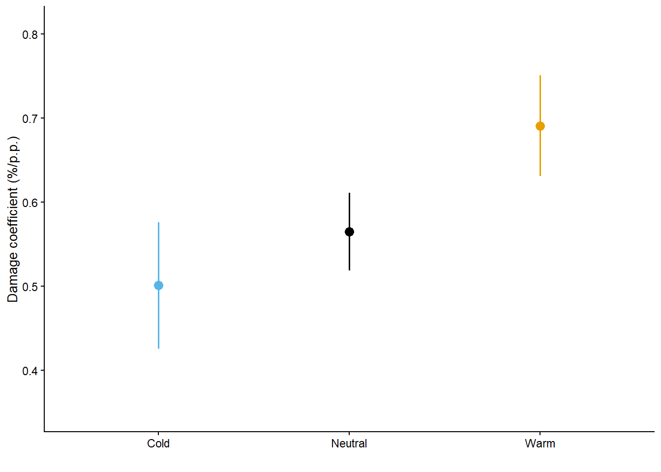

Yield loss

damage_coef_df =as.data.frame(emmeans(grid,specs = ~enso)) |> 
    mutate(enso = factor(enso, levels = c("Neutral",  "Warm","Cold"))) |> 
  mutate(`100` = 100-100*emmean,
         `0` = 100,
         `50` = 100-50*emmean,
         `50_upper` = 100-50*lower.CL,
         `50_lower` = 100-50*upper.CL) |>
  mutate(yield_50 = 100-50*emmean) 

damage_coef_df_for_plot = damage_coef_df|>
  pivot_longer(7:8,
               names_to = "sev", 
               values_to = "yloss") %>%
  mutate(sev = as.numeric(sev)) %>%
  mutate(cil = 100-sev*lower.CL,
         ciu = 100-sev*upper.CL) |> 
  mutate(yl = -(yloss-100)) 
  
rel_gg = damage_coef_df_for_plot |> 
  ggplot()+
  geom_ribbon(aes(x= sev,ymin = cil, ymax = ciu,  fill = enso ),alpha = 0.5, color = NA)+
  geom_line(aes(sev, yloss, color = enso),size = 1)+
  geom_vline(xintercept =50, linetype = "dashed", color = "gray40", size = 0.2)+
  geom_hline(aes(yintercept = yield_50, color = enso), linetype = "dashed", size = 0.2)+
  geom_point(aes(x = 50, y = yield_50, fill =enso ), size = 2, shape = 21, color = "white")+
  geom_label_repel(data = damage_coef_df,
                   aes(x =50, y = yield_50, fill =enso, label = paste0("Yield = ", round(yield_50,1),"%")),
                   label.size = 0.1, 
                   size = 2, 
                   color = "white",
                   seed = 123,
                   show.legend = F)+
  guides(text = F)+
  scale_linetype_manual(values = 2)+
  scale_color_colorblind()+
  scale_fill_colorblind()+
  scale_x_continuous(limits = c(0,100))+
  scale_y_continuous(limits = c(0,100), breaks = c(seq(0,100,by = 20)),
                     )+
  theme(strip.background = element_blank(),
        legend.position = "top")+
  coord_equal()+
  labs(x = "SBR Severity (%)",
       y = "Soybean yield (%)",
       color = "",
       fill = "")

Warning: The `<scale>` argument of `guides()` cannot be `FALSE`. Use "none" instead as
of ggplot2 3.3.4.

rel_gg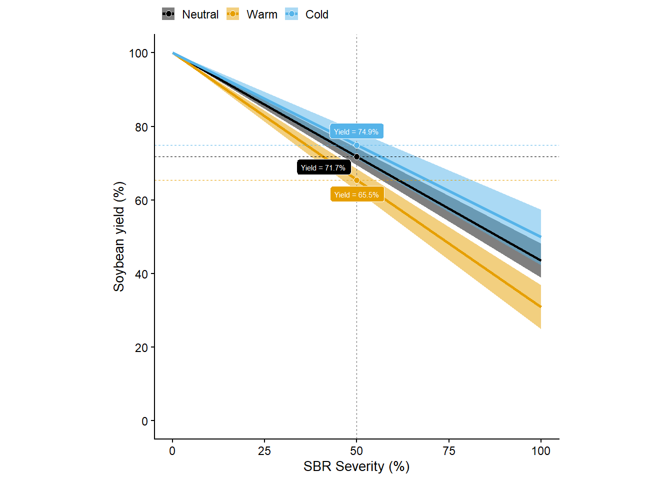

Combo plot

 (DC_gg+rel_gg)+
  plot_annotation(tag_levels = "a")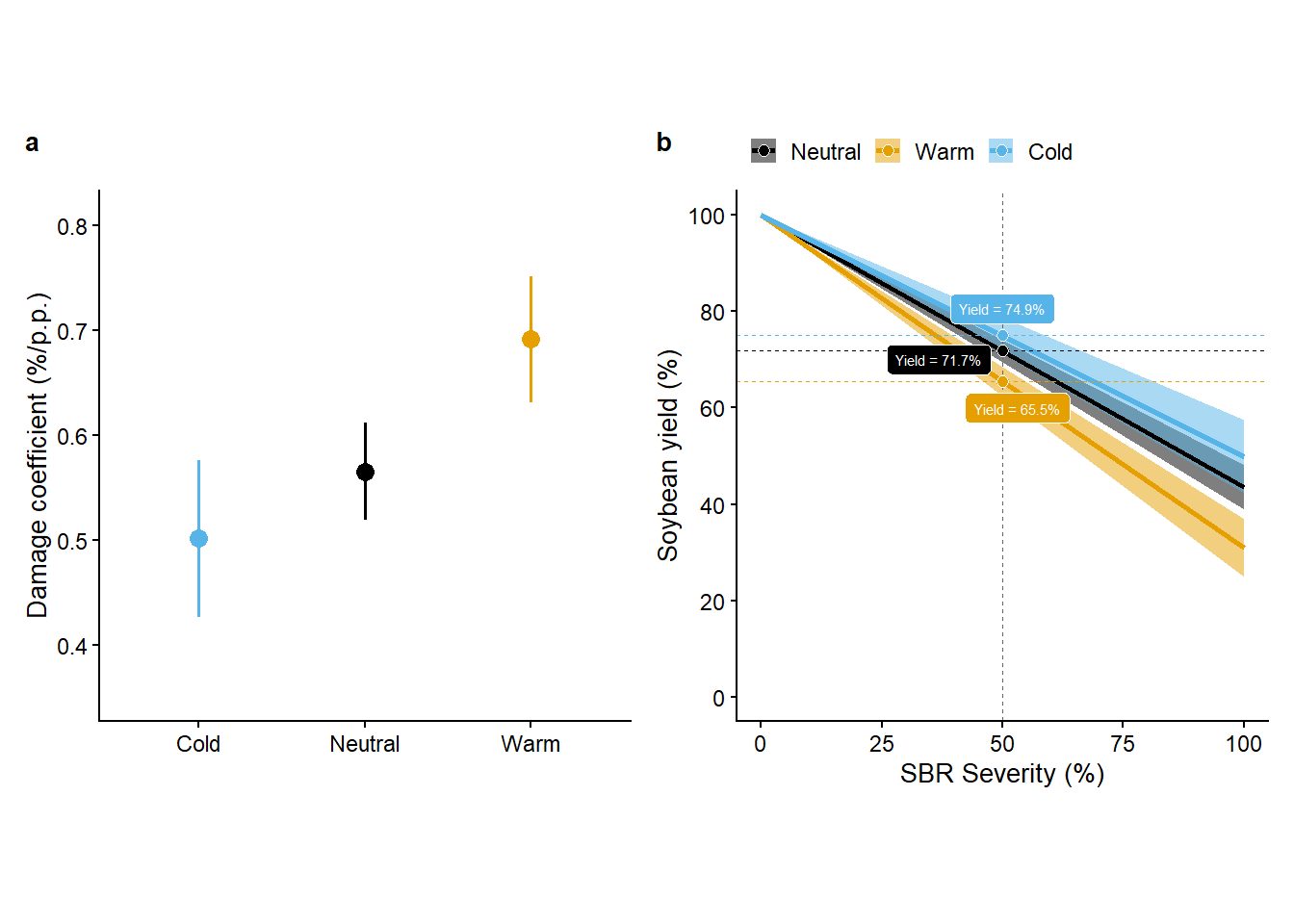

  # 
  # plot_layout(guides = "collect") &
  # theme(axis.title = element_text(size = 5),
  #       legend.position = "bottom")
  
  
ggsave("figs/z.png", dpi = 900, width =6, height = 3.5, bg ="white")
ggsave("figs/z.pdf", dpi = 900, width =6, height = 3.5, bg ="white")

Yield protection

Vector for attainable yield (ymax), control efficacy (lambda), severity in untreated field (sn), and damage coefficient (a).

length_grid = 500
ymax = seq(1500, 4000,length.out = length_grid) # attainable yield
lambda = c(30, 50, 70) # control efficacy
sn = seq(0, 100,length.out = length_grid) # seveiry on untreated
a = dc_data$emmean # damage coeficients

Calculating yield protection (yld_protection) for the grid of vectors

yprotection_df = expand.grid(ymax = ymax,lambda = lambda, sn = sn, a = a) |> 
  mutate(yld_protection = ((a*ymax)/100) *(sn-(sn*(1-lambda/100)))) |> 
  mutate(lambda = paste0(lambda,"% of Control")) |> 
  full_join(dc_data |> rename(a = emmean))

Joining with `by = join_by(a)`

Response surfaces

Absolute yield protection

yprotection_df |> 
  ggplot(aes(sn, ymax, fill = yld_protection))+ 
  geom_raster()+
  scale_fill_viridis_b(option = "A", 
                       guide = guide_colorbar(barwidth = 15, barheight = 0.3),
                       breaks = seq(0, 3000, by =250)
                       )+
  facet_grid(lambda~enso)+
  scale_y_continuous(breaks = seq(min(ymax), max(ymax), length.out = 5))+
  theme_minimal_grid(font_size = 10)+
  labs(y = "Attainable yield (kg/ha)",
       x = "Severity untreated (%)",
       fill ="Yield protection (kg/ha)" )+
  theme(panel.grid = element_blank(),
        axis.text = element_text(size = 5),
        legend.position = "bottom")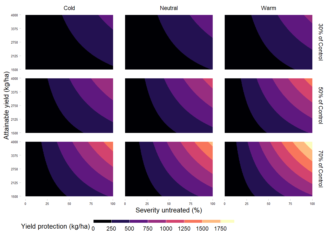

ggsave("figs/surface_yield_protection.png", dpi = 600,height =5, width = 5, bg = "white" )

Yield protection difference from Neutral ENSO

yprotection_df_diff = yprotection_df |> 
  group_by(enso) |> 
  mutate(id = 1:length(enso)) |> 
  ungroup() |> 
  pivot_wider(id_cols = c(id,lambda, sn,ymax),
              values_from = yld_protection,
              names_from = enso) |> 
  mutate(Cold = Cold - Neutral,
         Warm = Warm -Neutral) |> 
  dplyr::select(-Neutral) |> 
  pivot_longer(5:6,
               values_to = "diff",
               names_to = "enso")
max(yprotection_df_diff$diff)

[1] 352.3533

yprotection_df_diff |> 
  ggplot(aes(sn, ymax, fill = diff))+ 
  geom_raster()+
  scale_fill_steps2(midpoint = 0,
                    low = "#742881ff",#"#",
                    mid = "#f9f9f9ff",
                    high = "#1b7939ff",#"#27456e",
                    guide = guide_colorbar(barwidth = 10, barheight = 0.3),
                    limits = c(min(yprotection_df_diff$diff),max(yprotection_df_diff$diff)),
                    breaks = seq(-200, 350, by =50))+
  scale_y_continuous(breaks = seq(min(ymax), max(ymax), length.out = 5))+
  scale_x_continuous(breaks = seq(min(sn)*100, max(sn)*100, length.out = 5 ))+
  facet_grid(lambda~enso)+
  theme_minimal_grid(font_size = 10)+
  labs(y = "Attainable yield (kg/ha)",
       x = "Severity untreated (%)",
       fill ="Difference in yield protection\nfrom neutral ENSO phase (kg/ha)" )+
  theme(panel.grid = element_blank(),
        legend.position = "bottom",
        axis.text = element_text(size =8),
        legend.text = element_text(size =6),
        legend.title = element_text(size =6))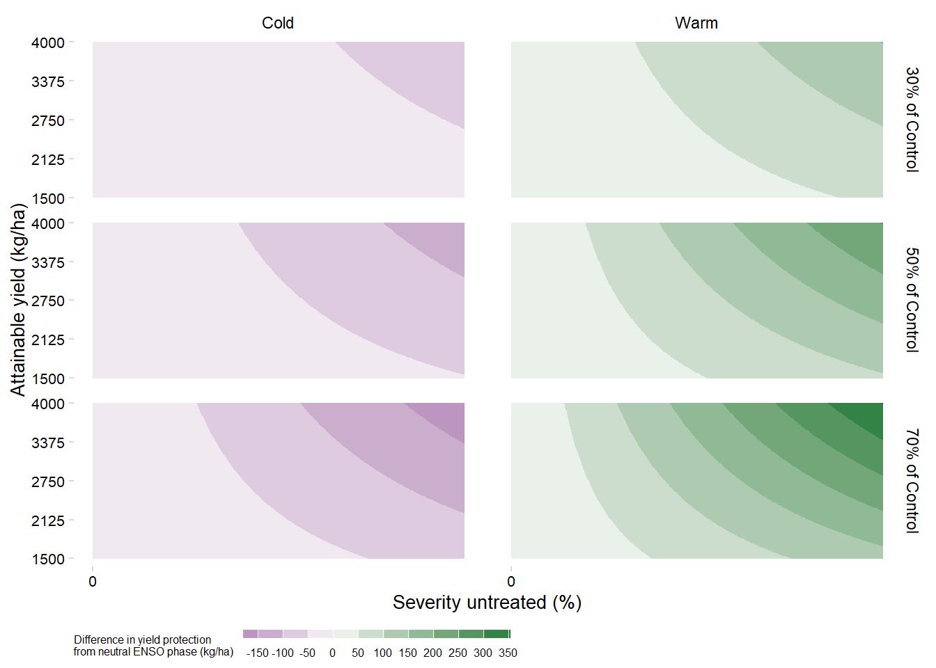

ggsave("figs/surface_yield_protection_difference.png", dpi = 600, height =5, width = 4, bg = "white" )
ggsave("figs/surface_yield_protection_difference.pdf", dpi = 600, height =5, width = 4, bg = "white" )

expand.grid(a = seq(0.1, 1, length.out = 20),
            sev = seq(0,100,by =5 ),
            lambda = c(50, 70),
            ymax = ymax[250])|> 
  mutate(yld_protection = (a*ymax*(sev - sev*((1-lambda/100))))/100) |> 
  ggplot(aes(sev, yld_protection, group = a, color = a))+
  geom_line(size = 1)+
  scale_color_viridis_c()+
  facet_rep_wrap(~lambda)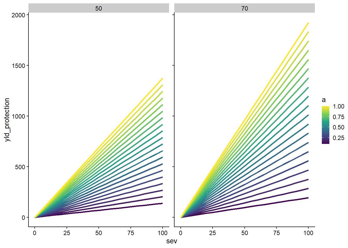

Session Info

sessionInfo()

R version 4.4.1 (2024-06-14 ucrt)
Platform: x86_64-w64-mingw32/x64
Running under: Windows 11 x64 (build 26100)

Matrix products: default


locale:
[1] LC_COLLATE=Portuguese_Brazil.utf8  LC_CTYPE=Portuguese_Brazil.utf8   
[3] LC_MONETARY=Portuguese_Brazil.utf8 LC_NUMERIC=C                      
[5] LC_TIME=Portuguese_Brazil.utf8    

time zone: America/Sao_Paulo
tzcode source: internal

attached base packages:
[1] stats     graphics  grDevices datasets  utils     methods   base     

other attached packages:
 [1] scales_1.3.0        minpack.lm_1.2-4    metafor_4.6-0      
 [4] numDeriv_2016.8-1.1 metadat_1.2-0       ggthemes_5.1.0     
 [7] multcomp_1.4-26     TH.data_1.1-2       MASS_7.3-60.2      
[10] survival_3.6-4      mvtnorm_1.3-2       emmeans_1.10.6     
[13] lmerTest_3.1-3      ggrepel_0.9.6       ggforce_0.4.2      
[16] lme4_1.1-35.5       Matrix_1.7-0        lemon_0.4.9        
[19] patchwork_1.3.0     cowplot_1.1.3       gsheet_0.4.6       
[22] lubridate_1.9.3     forcats_1.0.0       stringr_1.5.1      
[25] dplyr_1.1.4         purrr_1.0.2         readr_2.1.5        
[28] tidyr_1.3.1         tibble_3.2.1        ggplot2_3.5.1      
[31] tidyverse_2.0.0    

loaded via a namespace (and not attached):
 [1] gridExtra_2.3        gld_2.6.6            sandwich_3.1-1      
 [4] readxl_1.4.3         rlang_1.1.4          magrittr_2.0.3      
 [7] e1071_1.7-16         compiler_4.4.1       mgcv_1.9-1          
[10] systemfonts_1.1.0    vctrs_0.6.5          quadprog_1.5-8      
[13] pkgconfig_2.0.3      fastmap_1.2.0        backports_1.5.0     
[16] labeling_0.4.3       utf8_1.2.4           rmarkdown_2.28      
[19] tzdb_0.4.0           haven_2.5.4          nloptr_2.1.1        
[22] ragg_1.3.3           xfun_0.48            jsonlite_1.8.9      
[25] tweenr_2.0.3         broom_1.0.7          parallel_4.4.1      
[28] DescTools_0.99.58    R6_2.5.1             stringi_1.8.4       
[31] boot_1.3-30          cellranger_1.1.0     estimability_1.5.1  
[34] Rcpp_1.0.13          knitr_1.48           zoo_1.8-12          
[37] splines_4.4.1        timechange_0.3.0     tidyselect_1.2.1    
[40] rstudioapi_0.17.0    yaml_2.3.10          codetools_0.2-20    
[43] lattice_0.22-6       plyr_1.8.9           withr_3.0.2         
[46] evaluate_1.0.1       proxy_0.4-27         polyclip_1.10-7     
[49] ggdist_3.3.2         pillar_1.9.0         BiocManager_1.30.25 
[52] renv_1.1.2           distributional_0.5.0 generics_0.1.3      
[55] mathjaxr_1.6-0       hms_1.1.3            munsell_0.5.1       
[58] rootSolve_1.8.2.4    minqa_1.2.8          class_7.3-22        
[61] glue_1.8.0           lmom_3.2             tools_4.4.1         
[64] data.table_1.16.2    Exact_3.3            grid_4.4.1          
[67] colorspace_2.1-1     nlme_3.1-164         cli_3.6.3           
[70] textshaping_0.4.0    fansi_1.0.6          expm_1.0-0          
[73] viridisLite_0.4.2    gtable_0.3.5         digest_0.6.37       
[76] pbkrtest_0.5.4       farver_2.1.2         htmltools_0.5.8.1   
[79] lifecycle_1.0.4      multcompView_0.1-10  httr_1.4.7

Introduction

Getting started

Prerequisites

Steps to Initialize the Environment

Running the Analysis

Packages

Data

Soybean Rust data

ENSO data

Data wrangling

Tranformations

Exploratory analysis

Average, min and max severity

Overal

by year

By ENSO state

plot

Graph over time

Average, min and max yield

Overal

by year

By ENSO state

Modeling Severity (untreated) and ENSO

Mixed-effect model

Model summary

Pairwise comparison

All Severity data (plot)

Modeling soybean yield and ENSO

Graph over time

Mixed-effect model

Model summary

Pairwise comparison

All yield data

Graph over time

Combo plot

Modeling disease damage

Yield vs. Severity

Meta-analysis

Ordinary Regression

Graph of the regression lines

Distribution of intercepts and slopes

Relative yield loss (%) relative to β0

Second Regression l ~ 0 + sev

Damage vs. ENSO phases

Combo plot

Meta-analytical model

Estimates for each moderator

Graphs

Forest plot

Damage coefficient

Yield loss

Combo plot

Yield protection

Response surfaces

Absolute yield protection

Yield protection difference from Neutral ENSO

Session Info

Relative yield loss (%) relative to β₀